DeepONet and Operator Learning
Published:
Conventional trials of physics-informed deep learning (say, PINNs) integrates the dynamics as constraints to guide the approximation of a certain function within. An obvious problem with this idea is that such models cannot be directly applied to different initial and boundary conditions and observations. DeepONet, representing a new trial in physics-informed learning, employed some tricks to get around with this.
Start from Operator
The letter O in DeepONet refers to operator, which maps between infinite-dimensional function spaces. One example of it is given below, along with one of function for the convenience of comparison.
- Function: maps between vector spaces, e.g., $f_1(x)=\sin(x), x\in \mathbf{R}$, in other words $f_1$ maps $\mathbf{R}\rightarrow [0, 1]$
- Operator: maps between infinite-dimensional function spaces $G(f_1(x))=f_2(x)$, e.g., derivative operator $\frac{\mathrm{d}}{\mathrm{d}x}$ which can transform a function $f_1$ to another $f_2$.
So why and how is operator introduced in this work? In this section, we may look at the “why” question first.
To solve PDEs in real world, we may have an overall unified governing framework with varying coefficients and boundary conditions. The model trained to fit a solution within one scenario is likely not to generalize well over other ones.
Let $\mathcal{N}$ be a nonlinear derivative operator, we have a general representation of PDEs
\(\mathcal{N}(u, s)=0,\) where $u$ is the input function, while $s$ is the unknown PDE’s solution (also a function). Then the solution operator will be \(G(u)=s.\) Note that since $s$ is itself a function, so if we evaluate it at any point $y$, the answer will be a real number \(G(u)(y)=s(y)\in \mathbf{R}.\) If we can fit the operator $G$, then the model should in principle have better generalization ability for various inputs $u$. This is where operator learning differs from PINNs.
Universal Approximation for Operators
For function approximation, there is a prestigious universal approximation theorem that has been heavily studied. What about operators? Here are also 2 for them.
- Suppose that $\sigma$ is a continuous non-polynomial function, $X$ is a Banach space, $K_1\subset X$, $K_2\subset \mathbb{R}^d$ are two compact sets in $X$ and $\mathbb{R}^d$, V is a compact set in $C(K_1)$, $G$ is a nonlinear continuous operator that maps $V$ into $C(K_2)$. Then for any $\epsilon>0$, there are positive integers $n, p, m$, constants $c_i^k, \xi_{ij}^k, \theta_i^k, \zeta_k \in \mathbb{R}, w_k \in \mathbb{R}^d, i=1,\dots,n, k=1,\dots,p, j=1,\dots,m$ such that
holds for any $u\in V$ and $y\in K_2$. Here $C(K)$ is the Banach space of all continuous functions defined in $K$, whose norm is given by
\[\left|f\right|_{C(K)}=\max_{x\in\mathbb{K}}\left|f(x)\right|^\prime.\]- Suppose that $X$ is a Banach space, $K_1\subset X$, $K_2\subset \mathbb{R}^d$ are two compact sets in $X$ and $\mathbb{R}^d$, V is a compact set in $C(K_1)$, $G$ is a nonlinear continuous operator that maps $V$ into $C(K_2)$. Then for any $\epsilon>0$, there are two positive integers $m, p$, continuous vector functions $\mathbf{g}: \mathbb{R}^m \Rightarrow \mathbb{R}^p$ and $\mathbf{g}: \mathbb{R}^d \Rightarrow \mathbb{R}^p$, and $x_1, x_2, \dots, x_m\in K_1$ such that
holds for any $u\in V$ and $y\in K_2$. $\langle\cdot, \cdot\rangle$ represents the inner product of vectors. With limited space, proofs wll not be elaborated here.
DeepONet
With the theorems above, we can easily regard $\sigma$, $g$ and $f$ as neural networks with parameters to be estimated. This is the general idea of DeepONet, and we can see from the figure below.
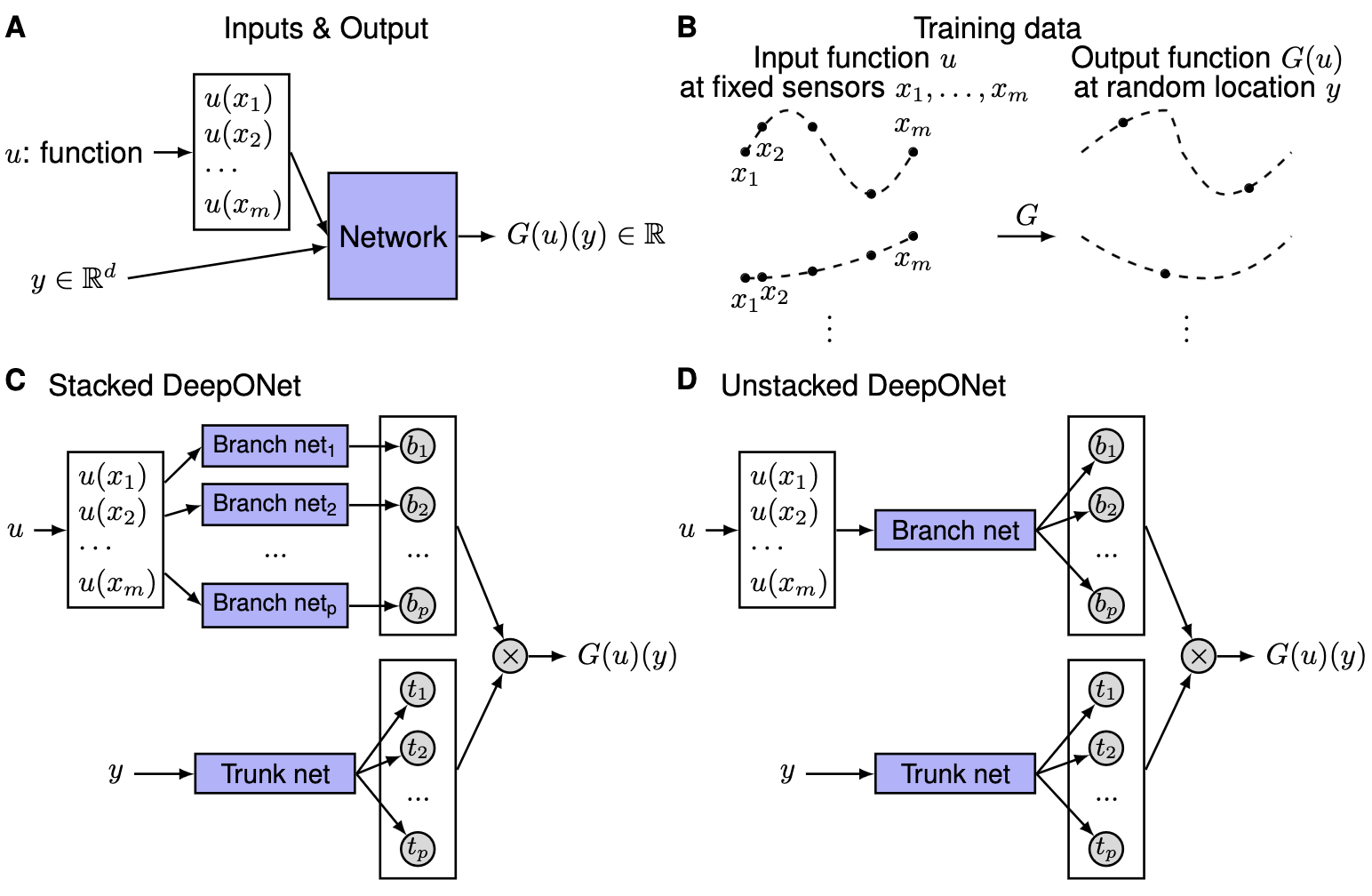 Here A) dircetly use the value of $u$ at fixed points $x_1, x_2, \dots, x_m$ and $y$ as inputs, and then outputs the predicted $G(u)(y)$. This design may be theoretically feasible, yet absolutely difficult to train. B) illustrates what input and output should look like in an intuitive way. C) and D) are stacked and unstacked DeepONet architectures repsectively. Following the approximation theorems, they both contain branch net and trunk net, and the only difference is that the unstacked version shares the same parameter for encoding $u$.
The loss function for DeepONet is given by
\[\mathcal{L}(\boldsymbol{\theta})=\lambda_{i c} \mathcal{L}_{i c}(\boldsymbol{\theta})+\lambda_{b c} \mathcal{L}_{b c}(\boldsymbol{\theta})+\lambda_r \mathcal{L}_r(\boldsymbol{\theta})+\lambda_g \mathcal{L}_g(\boldsymbol{\theta}),\]with each term expanding as
\[\begin{gathered} \mathcal{L}_{i c}(\boldsymbol{\theta})=\frac{1}{N_{i c}} \sum_{i=1}^{N_{i c}}\left|\boldsymbol{u}_{\boldsymbol{\theta}}\left(0, \boldsymbol{x}_{i c}^i\right)-\boldsymbol{g}\left(\boldsymbol{x}_{i c}^i\right)\right|^2 \\ \mathcal{L}_{b c}(\boldsymbol{\theta})=\frac{1}{N_{b c}} \sum_{i=1}^{N_{b c}}\left|\mathcal{B}\left[\boldsymbol{u}_{\boldsymbol{\theta}}\right]\left(t_{b c}^i, \boldsymbol{x}_{b c}^i\right)\right|^2 \\ \mathcal{L}_r(\boldsymbol{\theta})=\frac{1}{N_r} \sum_{i=1}^{N_r}\left|\frac{\partial \boldsymbol{u}_{\boldsymbol{\theta}}}{\partial t}\left(t_r^i, \boldsymbol{x}_r^i\right)+\mathcal{N}\left[\boldsymbol{u}_{\boldsymbol{\theta}}\right]\left(t_r^i, \boldsymbol{x}_r^i\right)\right|^2 \\ \mathcal{L}_g(\boldsymbol{\theta})=\frac{1}{P N_g} \sum_{j=1}^P \sum_{i=1}^{N_g}\left|\boldsymbol{u}_{\boldsymbol{\theta}}\left(t_r^j, \boldsymbol{x}_g^i\right)-\boldsymbol{u}_g\left(t_r^j, \boldsymbol{x}_g^i\right)\right|^2. \end{gathered}\]Herein \(\mathcal{L}_{ic}\) denotes the discrepancy between real and predicted values under initial conditions, \(\mathcal{L}_{bc}\) the discrepancy between real and predicted values under boundary conditions, \(\mathcal{L}_{r}\) the constraints from the original PDE, and \(\mathcal{L}_{g}\) the discrepancy between ground truth observations and predictions. This part of DeepONet is somewhat similar to PINNs.