Mainstream AIGC models, like ChatGPT and Stable Diffusion, have been drawing much attention over the recent years. Despite the massive amount of high-quality dataset, advanced network structure and loads of GPUs, one innegligible factor that contributes to their success is the use of RLHF, or reinforcement learning from human feedback. This blog is mostly based on a paper in May 2023 by the Levine Lab at UCB, and probes into how RLHF can be elegantly integrated into diffusion framework.

• Basics
  • Diffusion
  • RLHF
• Integration: DDPO

Basics

Before we start, we may as well have a grasp of what is diffusion model and RLHF, and how they work.

Diffusion

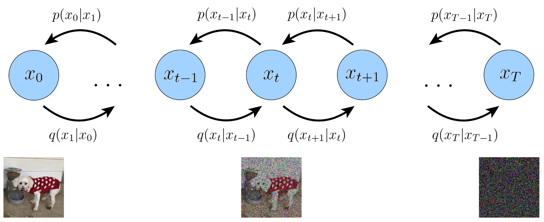
On the basis of its daily usages, diffusion model learns to generate images via first gradually adding Gaussian noise to an original one until completely destroying it and turning it into a pure Gaussian noise, and then trying to recover the image from the noise. Unlike popular choices for generative tasks in the past like GAN, diffusion provides an unsupervised, or more exactly, self-supervised manner of training, which is less demanding since there is no need for a data pair with extra annotation workload.

More generally, diffusion model leans a mapping that can go from a starting probability density function (PDF, usually Gaussian) to, theoretically, a desired, arbitrary one. My blog post back in Oct. last year have provided some interesting insights into approximating a PDF via score-matching, which is a less usual perspective for understanding diffusion models. Have a look if you’re interested.

RLHF

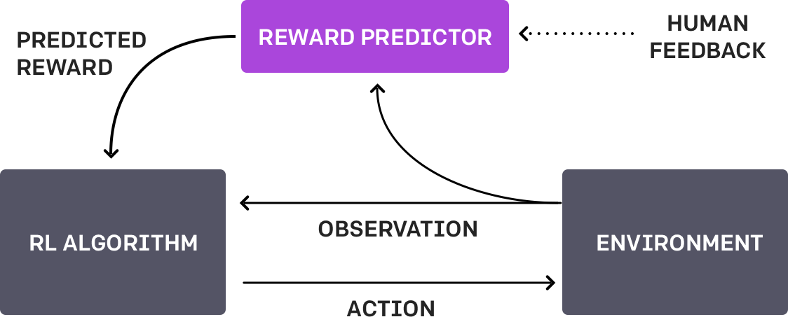
As its name suggests, RLHF aims to align an intelligent agent’s perception to human preferences via the paradigm of RL, using human feedback as at least part of its supervision. The intelligent agent is usually a pretrained generative model, and an extra reward model is trained on human feedbacks collected that are for the samples generated by the pretrained model, or we can simply integrate human feedbacks into the RL system as rewards - as long as you don’t mind heavy labelling of each sample generated. And this is why I say “part of” - to promote efficiency, the popular choice is to train a reward model that can mimic human perception as reliable as possible.

Currently popular generative models, despite their prowess to generate visually realistic images, texts, etc., still fail to provide serious productivity that can be much more meaningful and exacting than entertainment, especially for safe-sensitive applications like medical imaging. One possible workaround may lie in improvement of the design of training loss. Most diffusion models, for example, utilize MSE as their loss function, and it often leads to oversmoothing particularly when the number of training epochs is not large enough. However, to design a loss function that can offer very human-like assessment for the samples, and at the same time is differentiable and easy to compute for optimization of the model, is outrageously difficult. Perceptual loss may be one feasible option, but aligning feature maps cannot guarantee the model’s similarity to how human feel about the samples - how can we know the “feature map” in our brain?

Out of this concern, RLHF seems to be a solution that is not perfect, but at least better - how about using human ourselves as supervision, and modeling our response and comments to the model’s inference as some kind of reward. Then the idea of RL can be brought in here.

Integration: DDPO

For a model with parameter $\theta$, the goal is to maximize the reward signal, i.e.,

Herein $\mathbf{c}$ is the condition for our diffusion model, and $r(\cdot)$ is the reward function. One na"ive way to combine the goal with diffusion optimization may be a single evaluation and then backpropagation. However, recall the denoising procedure of a diffusion model, and we can find that it contains multiple timesteps. This can be regarded as a trajectory, a concept defined in RL that consists of a series of states ad actions. To embed the diffusion denoising procedure into RL framework, we need to first formulate a corresponding MDP for it.

• State: the current noisy image $\mathbf{s}=\mathbf{x}_t$.
• Action: the next denoised image $\mathbf{a}=\mathbf{x}_{t-1}$
• Policy: \(\pi(\mathbf{a}_t\mid \mathbf{s}_t)=p^{\text{diffusion}}_\theta\left(\mathbf{x}_{t-1} \mid \mathbf{x}_t, \mathbf{c}\right)\) decides the next action given the current state, exactly what we want to optimize.
• Reward: see below; after each action/state, zero until the last step of denoising is complete.

Then the entire trajectory can be presented as $\tau$. The optimization goal is then written as

With the formulation above, now policy gradient optimization methods can be applied. Let’s start from REINFORCE. Diffusion models can generally serve as score function estimator, and the score estimator of an arbitrary function $f(\mathbf{x})$ is written as

Combined with the MDP framework, the policy gradient can be given by

This gradient is usually referred to as the REINFORCE gradient, and with this, we can update our model via gradient ascent

However, the expectation $\mathbb{E}{\tau \sim p\theta(\tau)}$ is for all possible trajectories and we cannot take all of them. So it should be estimated with only the sampled trajectories in the current batch instead. Also, a loss function can be constructed from the gradient given above

and then we don’t need to calculate the gradient and pass it to the optimizer manually. One intuition is that, the loss function looks like a negative log-likelihood function, with actions as the targets. The difference lies in that it is weighted by the rewards. The loss then, as you can guess, tries to lead the model on a high-reward trajectory.

Subtituting the notations with ones in the diffusion framework, we can get a more easy-to-understand objective for the optimization

One challenge with this approach is that for each optimization step, the sampling from the current iteration of the model needs to be performed, and we need to re-calculate $\mathbf{x}_t$ as it comes from the current version of the model. This is very computationally demanding and wasteful, as the samples collected with previous iterations of the model cannot be used to learn.

One trick to address this is known as importance sampling. This relies on the following identity

Applying importance sampling to the gradient, we have

Again, we replace the notations with ones from the diffusion framework and we have

Minimization of this loss function is equivalent to gradient with the following gradient

Note that reward $r(\mathbf{x}_0,\mathbf{c})$ is usually normalized in practice to provide better convergence, and the normalized version is called advantage $A(\mathbf{x}_0, \mathbf{c})$¹. In addition, we don’t want current policy diverge too much from the previous policy, otherwise chances are that we may diverge and get a bad policy. So clipping is adopted for the sampling ratio of the loss function.

The loss function can be written in a way that’s numerically easier to calculate/more stable (using logs, ignoring the clipping for now)