Integro-Differential Equations and Neural Network
Published:
Integro-Differential Equations, IDEs for short, are equations involving both partial differential and integral operators. They are commonly used in a variety of disciplines of science and engineering topics, while nonlinear IDEs are particularly difficult to solve analytically. Therefore, the idea to incorporate neural networks arises naturally. This post is dedicated to recording my understanding of IDEs and NNs.
To Start With: IDEs
An IDE typically involves both integrals and derivatives of a function. For example, a general first-order, linear IDE is written as
\[\nabla_x u(x)+\int_{x_0}^xf(t, u(t))\mathrm{d}t=g(x, u(x)), u(x_0)=u_0, x_0>0.\]For IDEs formulation in real-world problems, a closed-form solution could be intractable. And NN is one of the recent trials to approximate it.
NNs for IDEs
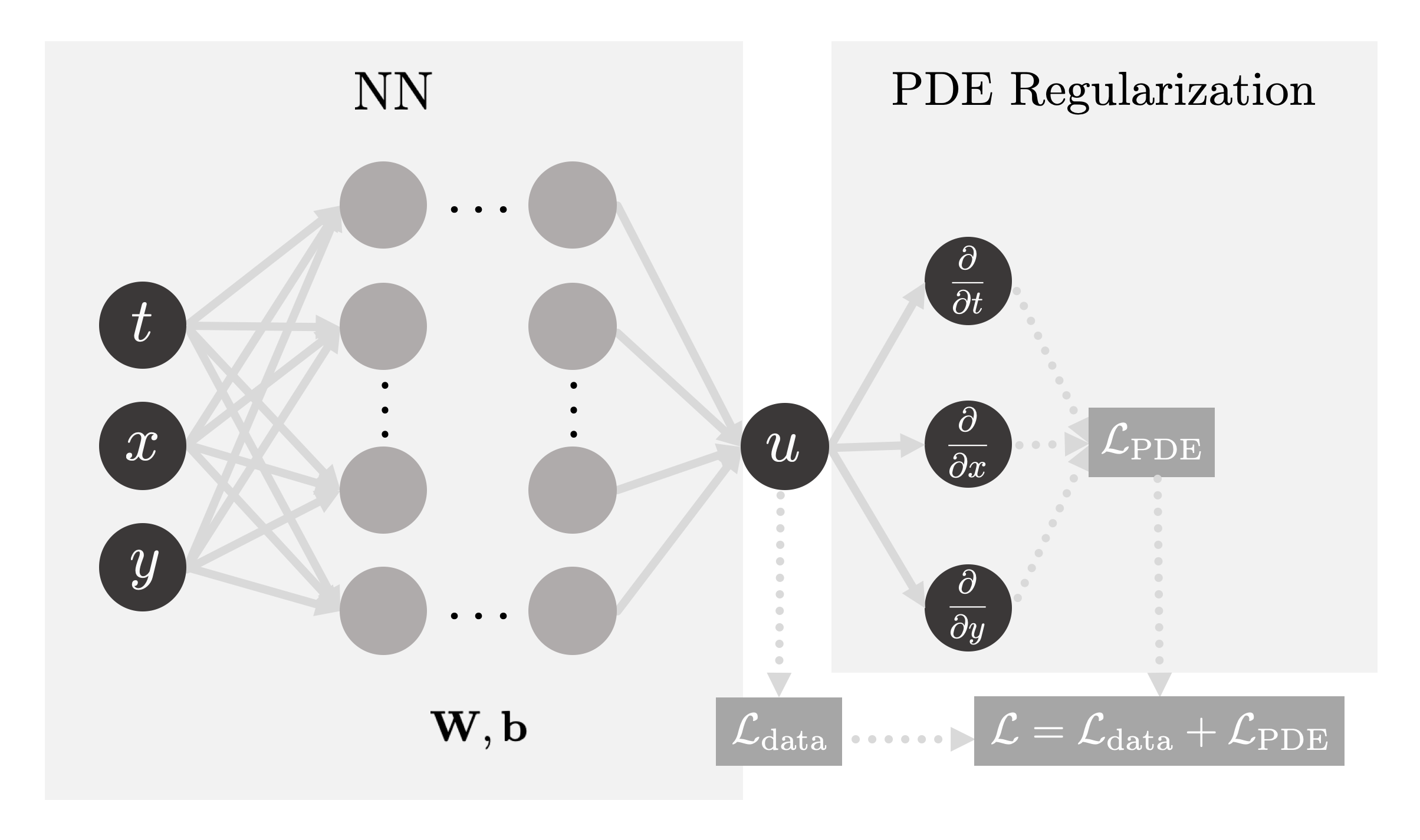
PINN for PDEs
Before diving into NN for IDEs, it’s important to first have a look at Physics Informed Neural Network (PINN). PINNs are a type of universal function approximators that can embed the knowledge of any physical laws that govern a given dataset in the learning process, and can be described by PDEs1. PDE-based physics are usually extremely difficult to simulate or solve, with generations of researchers trying to find algorithms with both better speed and accuracy, e.g., the notorious Navier-Stokes equation
\[\frac{\mathrm{D}\boldsymbol{u}}{\mathrm{D}t}=\frac{1}{\rho}\nabla\cdot \boldsymbol{\sigma}+\boldsymbol{g}.\]But as a novice, NS is not a good place to start; we are not learning fluid dynamics anyway. We may start with a general nonlinear PDE
\[u_t+\mathcal{N}[u; \lambda]0, x \in \Omega, t\in [0, T],\]where $u(t, x)$ denotes the solution, $\mathcal{N}[\cdot; \lambda]$ is a nonlinear operator parameterized by $\lambda$, and $\Omega$ is a subset of $\mathbb{R}^D$. However, sometimes it is not the dynamics $u(t, x)$ that we need, so below we have two sections for the typical two problems in a PDE system.
Forward Problem
Forward problem of PDEs computes the hidden state $u(t, x)$ of the system, given boundary conditions and/or measurements $z$, with fixed model parameter $\lambda$
\[u_t+\mathcal{N}[u]0, x \in \Omega, t\in [0, T],\]First, we define the residual $f(x, t)$ as
\[f := u_t+\mathcal{N}[u]=0,\]and the loss function comprises 2 parts,
\[\begin{aligned} L_{tot}&=L_u+L_f, \\ \text{where}\ L_u&=\|u-z\|_{\Gamma}\ \text{and} \\ L_f &= \|f\|_{\Gamma}. \end{aligned}\]$L_u$ is the error between PINN $u(t, x)$ and boundary conditions and measured data on data points $\Gamma$, and $L_f$ is the MSE error of the residual function, representing constraints from the governing equation itself.
Inverse Problem
Contrary to forward problem, Inverse ones not only require the system $u(t, x)$, but also the parameter $\lambda$, based on measurements $z$. So residual here is defined as
\[f := u_t+\mathcal{N}[u; \lambda]=0,\]and the rest is almost the same as above. The difference just lies in that the nonlinear operator $\mathcal{N}[\cdot; \lambda]$, characterized by $\lambda$, is unknown as well and needed to be solved.
A-PINNs for IDEs
As mentioned above, IDEs involve both integrals and gradients, and are thus even harder for conventional numerical methods. It is intuitive to use a neural network to represent the targeted dynamics, with its derivative as the gradient via automatic differentiation mechanism. The question is: how to approximate the integral?
One natural idea, called Auxiliary PINN (A-PINN), introduced by Yuan et al.2, is to model the integral itself as an auxiliary function approximated by a neural network. Thus its derivative is the integrand that could serve for some supervising purposes. For example, as is formulated in their paper, for the first-order nonlinear Volterra IDE
\[u^{(n)}(x)=f(x)+\lambda \int_0^x K(t) u(t) \mathrm{d} t, \quad u(0)=a.\]By defining an auxiliary function $v(x)$ to represent the integral, we have
\[\begin{aligned} u^{(n)}(x)&=f(x)+\lambda\cdot v(x)\\ v(x)&=\int_0^x K(t) u(t) \mathrm{d}t\\ u(0)&=a. \end{aligned}\]And the integral can be further re-expressed as
\[\begin{aligned} \nabla_x v(x)&= K(x)u(x)\\ v(0)&=0, \end{aligned}\]to avoid integral manipulation with the same ability to supervise our optimization. Thus far, it is clear that IDEs could be solved in a manner that is similar to PINNs: introducing an auxiliary function to replace the integral, turning the integral into its equivalent derivative form, and performing optimization with multiple governing PDEs and known measurements together. From a personal perspective, the idea of A-PINN is somewhat relevant to AutoInt, the automatic integration framework proposed by Lindell et al.3 Generally, they calculated the integral in the volume rendering equation by minimizing the discrepancy between its derivative/integrand and measurements, which is also how A-PINN deals with integrals in IDEs.
There have been attempts to employ A-PINN for IDEs like Boltzmann equation in radiative transfer problems4, and more exploration is certainly expected.
References
Raissi, Maziar, Paris Perdikaris, and George Em Karniadakis. “Physics informed deep learning (part i): Data-driven solutions of nonlinear partial differential equations.” arXiv preprint arXiv:1711.10561 (2017). ↩
Yuan, Lei, et al. “A-PINN: Auxiliary physics informed neural networks for forward and inverse problems of nonlinear integro-differential equations.” Journal of Computational Physics 462 (2022): 111260. ↩
Lindell, David B., Julien NP Martel, and Gordon Wetzstein. “Autoint: Automatic integration for fast neural volume rendering.” Proceedings of the IEEE/CVF Conference on Computer Vision and Pattern Recognition. 2021. ↩
Riganti, Roberto, and L. Dal Negro. “Auxiliary physics-informed neural networks for forward, inverse, and coupled radiative transfer problems.” Applied Physics Letters 123.17 (2023). ↩