Mathematical View of Generative Models
Published:
Generative models, powered by AI, is a big trend now for stuff synthesis (texts, images, and even more specialize usages). This post probes into why and how they are working from a mathematical perspective.
- To start with: Important Theorems \& Corollaries
- Denoising Diffusion Probabilistic Models
- Score-based Generative Models
- References
To start with: Important Theorems & Corollaries
Generally, in Bayesian inference, we would like to estimate parameter $\theta$ from observations $x$. For example, if we adopt MSE to measure the error between our estimation and the ground truth, then we have
\[L=\mathbb{E}[(\hat{\theta}(x)-\theta)^2],\]whose optimization equals to solving the expected value of the posterior distribution
\[\hat{\theta}(x)=\mathbb{E}[\hat{\theta}\mid x]=\int \theta \times p(\theta \mid x)\mathrm{d}x.\]Therefore, to estimate the parameter, posterior $p(\theta\mid x)$ is needed, which could be decomposed into a prior and a likelihood according to Bayes’s theorem. These are what we usually need for such estimation.
Tweedie Estimator
Here we suppose that the likelihood $p(x\mid \theta)$ conforms to a normal distribution, i.e.,
\[p(x\mid \theta)=\mathcal{N}(\mu, \sigma^2),\]and the marginal distribution $p(x)$ writes as follows
\[p(x)=\int^{\infty}_{-\infty}p(x\mid \theta)p(\theta)\mathrm{d}\theta.\]So we can derive
\[\begin{aligned} & \mathbb{E}[\theta \mid x]=\int_{-\infty}^{\infty} \theta p(\theta \mid x) \mathrm{d} \theta \\ & =\int_{-\infty}^{\infty} \theta \frac{p(x \mid \theta) p(\theta)}{p(x)} \mathrm{d} \theta \\ & =\frac{\int_{-\infty}^{\infty} \theta p(x \mid \theta) p(\theta) \mathrm{d} \theta}{p(x)} \\ & =\frac{\int_{-\infty}^{\infty} \theta \frac{1}{\sqrt{2 \pi \sigma^2}} e^{-\frac{(x-\theta)^2}{2 \sigma^2}} p(\theta) \mathrm{d} \theta}{p(x)} \\ & =\frac{\int_{-\infty}^{\infty}\left[\sigma^2 \frac{\theta-x}{\sigma^2} \frac{1}{\sqrt{2 \pi \sigma^2}} e^{-\frac{(x-\theta)^2}{2 \sigma^2}} p(\theta)+x \frac{1}{\sqrt{2 \pi \sigma^2}} e^{-\frac{(x-\theta)^2}{2 \sigma^2}} p(\theta)\right] \mathrm{d} \theta}{p(x)} \\ & =\frac{\int_{-\infty}^{\infty} \sigma^2 \frac{\theta-x}{\sigma^2} \frac{1}{\sqrt{2 \pi \sigma^2}} e^{-\frac{(x-\theta)^2}{2 \sigma^2}} p(\theta) \mathrm{d} \theta+\int_{-\infty}^{\infty} x \frac{1}{\sqrt{2 \pi \sigma^2}} e^{-\frac{(x-\theta)^2}{2 \sigma^2}} p(\theta) \mathrm{d} \theta}{p(x)} \\ & =\frac{\sigma^2 \int_{-\infty}^{\infty} \frac{\mathrm{d}\left[\frac{1}{\sqrt{2 \pi \sigma^2}} e^{-\frac{(x-\theta)^2}{2 \sigma^2}}\right]}{\mathrm{d} x} p(\theta) \mathrm{d} \theta+\int_{-\infty}^{\infty} x \frac{1}{\sqrt{2 \pi \sigma^2}} e^{-\frac{(x-\theta)^2}{2 \sigma^2}} p(\theta) \mathrm{d} \theta}{p(x)} \\ & =\frac{\sigma^2 \int_{-\infty}^{\infty} \frac{\mathrm{d} p(x \mid \theta)}{\mathrm{d} x} p(\theta) \mathrm{d} \theta+\int_{-\infty}^{\infty} x p(x \mid \theta) p(\theta) \mathrm{d} \theta}{p(x)} \\ & =\frac{\sigma^2 \frac{\mathrm{d}}{\mathrm{d} x} \int_{-\infty}^{\infty} p(x \mid \theta) p(\theta) \mathrm{d} \theta+x \int_{-\infty}^{\infty} p(x \mid \theta) p(\theta) \mathrm{d} \theta}{p(x)} \\ & =\frac{\sigma^2 \frac{\mathrm{d} p(x)}{\mathrm{d} x}+x p(x)}{p(x)} \\ & =x+\sigma^2 \frac{\mathrm{d}}{\mathrm{d} x} \log p(x) \\ & \end{aligned}\]Hitherto, it’s obvious that the posterior expectation bears no relevance to its prior distribution, and is merely related to the marginal distribution $p(x)$. So here we arrive at the Tweedie estimator
\[\hat{\theta}^{\text{TE}}=x+\sigma^2\frac{\mathrm{d}}{\mathrm{d}x}\log p(x)\]Score Matching
For an arbitrary distribution, there is a general form to represent it originating from energy-based model1.
\[p_{\theta}(x)=\frac{e^{-f_{\theta}(x)}}{Z(\theta)},\]where $Z(\theta)=\int e^{-f_{\theta}(x)}\mathrm{d}x$ is a constant for normalization, ensuring integral of the PDF $\int p_{\theta}(x)\mathrm{d}x=1$. For complex distributions, $Z(\theta)$ could be intractable, to circumvent which derivative is adopted instead.
\[\begin{aligned} \nabla_x \log p_{\theta}(x) &= \nabla_x \log e^{-f_{\theta}(x)}-\nabla_x \log Z(\theta)\\ &=-\nabla_x f_{\theta}(x)\\ &\approx s_{\theta}(x), \end{aligned}\]i.e., approximate the gradient of logarithm of the distribution by a neural network $s_{\theta}(x)$ with parameter $\theta$. $Z(\theta)$ has been zeroed out via gradient, thus leaving no effect on our estimation.
Score function is defined as the gradient of the logarithm of a distribution. And now we can perform optimization for a solution of targeted distribution
\[L=\mathbb{E}_{p(x)}[\|s_{\theta}(x)-\nabla_x \log p(x)\|_2^2]\]Generally, this is what score matching refers to: approximating the gradient of ground truth data distribution via matching that of predicted distribution to it.
To optimize the L2 loss above, gradient of the targeted distribution $p(x)$ with regard to data $x$ is needed. But usually we don’t know the true distribution, or it’s too sparse for calculating derivatives, therefore unable to supervise this optimization. We may need some further derivation.
\[\begin{aligned} L&=\mathbb{E}_{p(x)}[\|s_{\theta}(x)-\nabla_x \log p(x)\|_2^2]\\ &=\int p\left[\|\nabla_x \log p(x)\|^2-2\cdot \nabla_x\log p^T(x)\cdot s_{\theta}(x)+\|s_{\theta}(x)\|^2\right]\mathrm{d}x. \end{aligned}\]Since $L$ is a function of $\theta$, which is what we want to optimize, it’s apparent that the first term could be regarded as a constant and thus ignored. Now move on to the second term.
\[L_2=\int p(x)\nabla_x\log p^T(x)\cdot s_{\theta}(x)\mathrm{d}x.\]The 2 multiplied terms share the same number of dimensions. So obviously $L_2$ is a scalar, and since $x^T \cdot y=\sum_i x_iy_i$, we have
\[\begin{aligned} L_2&=\int p(x)\sum\limits_i\nabla_{x_i}\log p^T(x)\cdot s_{\theta}(x)\mathrm{d}x\\ &=\sum\limits_i\int p(x)\nabla_{x_i}\log p^T(x)\cdot s_{\theta}(x)\mathrm{d}x\\ &=\sum\limits_i\int p(x)\frac{\nabla_{x_i}p^T(x)}{p^T(x)}\cdot s_{\theta}(x)\mathrm{d}x\\ &=\sum\limits_i\int\nabla_{x_i}p^T(x)\cdot s_{\theta}(x)\mathrm{d}x\\ &=\sum\limits_i\int s_{\theta}(x)\mathrm{d}p(x)\\ &=\sum\limits_i(s_{\theta}(x)\cdot p(x)-\int p(x)\mathrm{d}s_{\theta}(x)). \end{aligned}\]Note that for a PDF $p(x)$, when $x\rightarrow \infty$, $p(x)\rightarrow 0$. So the first term in the deduction above can be zeroed out, and then we have
\[\begin{aligned} L_2&=\sum\limits_i\left(-\int p(x)\mathrm{d}s_{\theta}(x)\right)\\ &=-\sum\limits_i\int p(x)\nabla^2_{x_i}\log p_{\theta}(x)\mathrm{d}x. \end{aligned}\]So we need the second derivative for each i-th element, and $\sum_i$ here is apparently corresponds to the sum of diagonal of Hessian matrix. Note that the second derivative here equals to first derivative of our neural network, i.e.,
\[\nabla^2_{x_i}\log p_{\theta}(x)=\nabla_x s_{\theta}(x).\]To sum up, we arrive at the loss $L$ for score matching in its well-known form
\[L=\mathbb{E}_{p(x)}\left[\text{tr}(\nabla_x s_{\theta}(x))+\|s_{\theta}(x)\|^2_2\right].\]Thus far, it’s clear that knowledge about the ground truth data distribution $p(x)$ is no longer necessary when conducting score matching.
Langevin Dynamics
For non-French speaker, its pronunciation is close to /laŋˈjevɔn/.
Proposed by Paul Langevin, Langevin equation describes the dynamics of molecular systems2. Imagine the pollen grains on the surface of water: water molecules bumping into them from random directions, coercing them into random walk. Based on Newton’s law, it’s easy to write
\[\sum F=ma.\]And first, there is one factor known in $\sum F$: a random force $\epsilon_t$ given by water molecules, which could be hypothesized as a normal distribution, whose mean is 0 and whose variance increases as time goes by.
Besides, friction should be included: if one pollen grain has velocity in a given direction, there will be much more water molecules towards the front of it, slowing it down by friction. Therefore, it’s safe to say that the friction is inversely proportional to the grain’s velocity $v$, i.e., $-\gamma v$, where $\gamma$ is a friction coefficient.
Considering a generic $F$ for any possible external forces, now we arrive at
\[ma_t=-\gamma v_t + \epsilon_t + F\]This is usually called the underdamped form. Since pollen grains are pretty light, we may just leave out the term $ma_t$, thus arriving at the overdamped form
\[0=-\gamma v_t + \epsilon_t + F\]Force is a gradient of energy $E$ with regard to displacement $x$, and velocity is the derivative of displacement on time. So we can rewrite the formula above as
\[0=-\gamma \frac{\mathrm{d}x}{\mathrm{d}t} + \epsilon_t + \frac{\partial E}{\partial x}\]And we further discretize the time derivative and have
\[\begin{aligned} 0&=-\gamma \frac{x_{t+\mathrm{d}t}-x_t}{\mathrm{d}t} + \epsilon_t + \frac{\partial E}{\partial x}\\ \Rightarrow x_{t+\mathrm{d}t}&=x_t + \frac{\mathrm{d}t}{\gamma}\frac{\partial E}{\partial x} + \frac{\mathrm{d}t}{\gamma}\epsilon_t \end{aligned}\]Now recall how weights are updated in SGD
\[w_{t+1}=w_t-a \frac{\partial L}{\partial w_t}\]If we neglect the random term in Langevin dynamics, and compare the two equations, we can arrive at the following conclusions:
- displacement $x$ $\Longleftrightarrow$ weight $w$
- energy $E$ $\Longleftrightarrow$ loss $L$
- noise in Brownian motion $\Longleftrightarrow$ error of mini-batch
In this manner, it seems intuitive and reasonable that Langevin dynamics and SGD are analogous. If we combine SGD and Langevin dynamics, it’s basically adding Gaussian noise to the standard SGD, avoiding local optima, known as stochastic gradient Langevin dynamics3.
\[x_{t+1}\leftarrow x_t+\delta \nabla_x \log p(x_t)+\sqrt{2\delta}\epsilon_t, t=0, 1, \dots, T,\]where $x_0$ is sampled at random from a prior distribution, $\delta$ denotes step size, and $\epsilon_t\sim \mathcal{N}(0, \mathbf{I})$ is a perturbing term, ensuring that generated samples won’t collapse onto a mode, but hover around it for diversity. When $\delta\rightarrow 0$ and $T\rightarrow \infty$, the ultimate $x_t$ is just the real data.
Denoising Diffusion Probabilistic Models
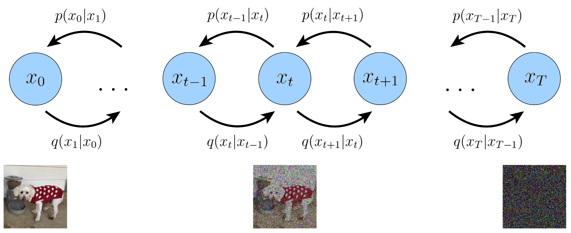
Forward Process: Adding Noise
$x_0$ is the original image, and each $x_{t-1}\rightarrow x_t$ adds noise gradually to it. Transitioning between 2 adjacent states can be modelled linearly, i.e.,
\[x_t=a_tx_{t-1}+b_t\varepsilon_t, \quad \varepsilon_t\sim \mathcal{N}(0, \mathbf{I})\]Obviously, since $x_{t-1}$ has more information, $a_t$ must be an attenuation coefficient, i.e., $a_t\in (0, 1)$. For simplicity, we may as well suppose that $b_t\in (0, 1)$. And now we expand the equation above as
\[\begin{aligned} x_t & =a_t x_{t-1}+b_t \varepsilon_t \\ & =a_t\left(a_{t-1} x_{t-2}+b_{t-1} \varepsilon_{t-1}\right)+b_t \varepsilon_t \\ & =a_t a_{t-1} x_{t-2}+a_t b_{t-1} \varepsilon_{t-1}+b_t \varepsilon_t \\ & =\ldots \\ & =\left(a_t \ldots a_1\right) x_0+\left(a_t \ldots a_2\right) b_1 \varepsilon_1+\left(a_t \ldots a_3\right) b_2 \varepsilon_2+\cdots+a_t b_{t-1} \varepsilon_{t-1}+b_t \varepsilon_t. \end{aligned}\]We can see that the besides the first term, the rest is the sum of multiple independent Gaussian noise, which is also a Gaussian distribution, whose mean is 0 and variance is the sum of squares of each coefficient $\left(a_t \ldots a_2\right)^2 b_1^2+\left(a_t \ldots a_3\right)^2 b_2^2+\cdots+a_t^2 b_{t-1}^2+b_t^2$. Therefore, it can be transformed into
\[x_t=\left(a_t \ldots a_1\right) x_0+\sqrt{\left(a_t \ldots a_2\right)^2 b_1^2+\left(a_t \ldots a_3\right)^2 b_2^2+\cdots+a_t^2 b_{t-1}^2+b_t^2}\bar{\varepsilon}_t, \\ \bar{\varepsilon}_t\sim \mathcal{N}(0, \mathbf{I}).\]Furthermore, if we add up the sum of squares of the coefficients, say,
\[\begin{aligned} & \left(a_t \ldots a_1\right)^2+\left(a_t \ldots a_2\right)^2 b_1^2+\left(a_t \ldots a_3\right)^2 b_2^2+\cdots+a_t^2 b_{t-1}^2+b_t^2 \\ = & \left(a_t \ldots a_2\right)^2 a_1^2+\left(a_t \ldots a_2\right)^2 b_1^2+\left(a_t \ldots a_3\right)^2 b_2^2+\cdots+a_t^2 b_{t-1}^2+b_t^2 \\ = & \left(a_t \ldots a_2\right)^2\left(a_1^2+b_1^2\right)+\left(a_t \ldots a_3\right)^2 b_2^2+\cdots+a_t^2 b_{t-1}^2+b_t^2 \\ = & \left(a_t \ldots a_3\right)^2\left(a_2^2\left(a_1^2+b_1^2\right)+b_2^2\right)+\cdots+a_t^2 b_{t-1}^2+b_t^2 \\ = & a_t^2\left(a_{t-1}^2\left(\ldots\left(a_2^2\left(a_1^2+b_1^2\right)+b_2^2\right)+\ldots\right)+b_{t-1}^2\right)+b_t^2 \end{aligned}\]it’s easy to simplify this term to $1$ when $a_t^2+b_t^2=1$. Denote $\bar{a}_t=(a_t\dots a_1)^2$, and then the variance can be written as $1-\bar{a}_t$. Then we further simplify the forward process to
\[x_t=\sqrt{\bar{a}_t}x_0+\sqrt{1-\bar{a}_t}\bar{\varepsilon_t}, \quad \bar{\varepsilon}_t\sim \mathcal{N}(0, \mathbf{I}).\]Then we rewrite Eq. (17) as follows,
\[x_t=\sqrt{a_t}x_0+\sqrt{1-a_t}\varepsilon_t, \quad \varepsilon_t\sim \mathcal{N}(0, \mathbf{I}),\]which aligns with the form in the original paper4. Utilizing techniques of re-parameterization, we could formulate the forward process as sampling from a Gaussian distribution, namely
\[x_t\sim q(x_t\mid x_{t-1})=\mathcal{N}(x_t; \sqrt{a_t}x_{t-1}, (1-a_t)\mathbf{I}).\]The whole forward process, thus, is an estimation of posterior, denoted as
\[q(x_{1:T}\mid x_0)=\prod\limits_{t=1}^T q(x_t\mid x_{t-1}).\]Backward Process: Removing Noise
The well-known generative model VAE encodes ($x\rightarrow z$) and decodes ($z\rightarrow x$) straightforward (encoder $q(z\mid x)$, decoder $p(x\mid z)$, and prior $q(z)$). This simpleness in turn limits its performance. Whereas diffusion model can be regarded as hierarchical VAE (HVAE), which decomposes the encode and decode processes into $T$ steps,
\[\begin{aligned} &\text{Encode}: x_0\rightarrow x_1\rightarrow x_2 \rightarrow \cdots \rightarrow x_T\\ &\text{Decode}: x_T\rightarrow x_{T-1}\rightarrow x_{T-2}\rightarrow \cdots \rightarrow x_0. \end{aligned}\]Each encode and decode sub-process can be modelled as $q(x_t\mid x_{t-1})$ and $p(x_{t-1}\mid x_t)$ respectively, which is similar to fitting a curve with piecewise function.
Generative models like VAE and diffusion model are all likelihood-based model, which, literally, maximizes the likelihood estimation $p_{\theta}(x_0)$ towards the real data distribution. Just like what we do in the forward process, we model each step of backward process as $p_{\theta}(x_{t-1}\mid x_t)$, and the linear relationship between 2 adjacent states as Gaussian distributions, i.e.,
\[p_{\theta}(x_{t-1}\mid x_t)=\mathcal{N}(x_{t-1};\mu_{\theta}(x_t, t), \Sigma_{\theta}(x_t, t)).\]And the whole backward process can be represented by a joint distribution
\[p_{\theta}(x_{0:T})=p(x_T)\prod_{t=1}^T p_{\theta}(x_{t-1}\mid x_t).\]Based on law of total probability, we can expand the logarithm of likelihood as follows
\[\begin{aligned} & \log p_{\theta}(x)=\log \int p_{\theta}\left(x_{0: T}\right) \mathrm{d} x_{1: T} \\ & =\log \int \frac{p_{\theta}\left(x_{0: T}\right) q\left(x_{1: T} \mid x_0\right)}{q\left(x_{1: T} \mid x_0\right)} \mathrm{d} x_{1: T} \\ & =\log \mathbb{E}_{q\left(x_{1: T} \mid x_0\right)}\left[\frac{p_{\theta}\left(x_{0: T}\right)}{q\left(x_{1: T} \mid x_0\right)}\right] \\ & \geq \mathbb{E}_{q\left(x_{1: T} \mid x_0\right)}\left[\log \frac{p_{\theta}\left(x_{0: T}\right)}{q\left(x_{1: T} \mid x_0\right)}\right] \\ & =\mathbb{E}_{q\left(x_{1: T} \mid x_0\right)}\left[\log \frac{p\left(x_T\right) \prod_{t=1}^T p_{\theta}\left(x_{t-1} \mid x_t\right)}{\prod_{t=1}^T q\left(x_t \mid x_{t-1}\right)}\right] \\ & =\mathbb{E}_{q\left(x_{1: T} \mid x_0\right)}\left[\log \frac{p\left(x_T\right) p_{\theta}\left(x_0 \mid x_1\right) \prod_{t=2}^T p_{\theta}\left(x_{t-1} \mid x_t\right)}{q\left(x_T \mid x_{T-1}\right) \prod_{t=1}^{T-1} q\left(x_t \mid x_{t-1}\right)}\right] \\ & =\mathbb{E}_{q\left(x_{1: T} \mid x_0\right)}\left[\log \frac{p\left(x_T\right) p_{\theta}\left(x_0 \mid x_1\right) \prod_{t=1}^{T-1} p_{\theta}\left(x_t \mid x_{t+1}\right)}{q\left(x_T \mid x_{T-1}\right) \prod_{t=1}^{T-1} q\left(x_t \mid x_{t-1}\right)}\right] \\ & =\mathbb{E}_{q\left(x_{1: T} \mid x_0\right)}\left[\log \frac{p\left(x_T\right) p_{\theta}\left(x_0 \mid x_1\right)}{q\left(x_T \mid x_{T-1}\right)}\right]+\mathbb{E}_{q\left(x_{1: T} \mid x_0\right)}\left[\log \prod_{t=1}^{T-1} \frac{p_{\theta}\left(x_t \mid x_{t+1}\right)}{q\left(x_t \mid x_{t-1}\right)}\right] \\ & =\mathbb{E}_{q\left(x_{1: T} \mid x_0\right)}\left[\log p_{\theta}\left(x_0 \mid x_1\right)\right]+\mathbb{E}_{q\left(x_{1: T} \mid x_0\right)}\left[\log \frac{p\left(x_T\right)}{q\left(x_T \mid x_{T-1}\right)}\right]+\mathbb{E}_{q\left(x_{1: T} \mid x_0\right)}\left[\sum_{t=1}^{T-1} \log \frac{p_{\theta}\left(x_t \mid x_{t+1}\right)}{q\left(x_t \mid x_{t-1}\right)}\right] \\ & =\mathbb{E}_{q\left(x_{1: T} \mid x_0\right)}\left[\log p_{\theta}\left(x_0 \mid x_1\right)\right]+\mathbb{E}_{q\left(x_{1: T} \mid x_0\right)}\left[\log \frac{p\left(x_T\right)}{q\left(x_T \mid x_{T-1}\right)}\right]+\sum_{t=1}^{T-1} \mathbb{E}_{q\left(x_{1: T} \mid x_0\right)}\left[\log \frac{p_{\theta}\left(x_t \mid x_{t+1}\right)}{q\left(x_t \mid x_{t-1}\right)}\right] \\ & =\mathbb{E}_{q\left(x_1 \mid x_0\right)}\left[\log p_{\theta}\left(x_0 \mid x_1\right)\right]+\mathbb{E}_{q\left(x_{T-1}, x_T \mid x_0\right)}\left[\log \frac{p\left(x_T\right)}{q\left(x_T \mid x_{T-1}\right)}\right]+\sum_{t=1}^{T-1} \mathbb{E}_{q\left(x_{t-1}, x_t, x_{t+1} \mid x_0\right)}\left[\log \frac{p_{\theta}\left(x_t \mid x_{t+1}\right)}{q\left(x_t \mid x_{t-1}\right)}\right] \\ & =\underbrace{\mathbb{E}_{q\left(x_1 \mid x_0\right)}\left[\log p_\theta\left(x_0 \mid x_1\right)\right]}_{\text {reconstruction term }}-\underbrace{\mathbb{E}_{q\left(x_{T-1} \mid x_0\right)}\left[D_{\mathrm{KL}}\left(q\left(x_T \mid x_{T-1}\right) \| p\left(x_T\right)\right)\right]}_{\text {prior matching term }} \\ & -\sum_{t=1}^{T-1} \underbrace{\mathbb{E}_{q\left(x_{t-1}, x_{t+1} \mid x_0\right)}\left[D_{\mathrm{KL}}\left(q\left(x_t \mid x_{t-1}\right) \| p_\theta\left(x_t \mid x_{t+1}\right)\right)\right]}_{\text {consistency term }}. \end{aligned}\]To calculate both $q\left(x_t \mid x_{t-1}\right)$ and $p_\theta\left(x_t \mid x_{t+1}\right)$ in the last consistency term demands knowledge of 3 random variables, which dramatically increases the variance of estimation. Note that currently the optimization means to minimize the discrepancy between real $x_t$ by adding forward noise to $x_{t-1}$ and estimated $x_t$ by removing noise backwardly from $x_{t+1}$.
Since $x_0$ is known and the steps are Markovian, we could have the following corollary.
\[q(x_t\mid x_{t-1}, x_0)=\frac{q(x_{t-1}\mid x_t, x_0)q(x_t\mid x_0)}{q(x_{t-1}\mid x_0)}.\]So we can rewrite the likelihood above as
\[\begin{aligned} \log p_{\theta}(x) & \geq \mathbb{E}_{q\left(x_{1: T} \mid x_0\right)}\left[\log \frac{p_{\theta}\left(x_{0: T}\right)}{q\left(x_{1: T} \mid x_0\right)}\right] \\ & =\mathbb{E}_{q\left(x_{1: T} \mid x_0\right)}\left[\log \frac{p\left(x_T\right) \prod_{t=1}^T p_{\theta}\left(x_{t-1} \mid x_t\right)}{\prod_{t=1}^T q\left(x_t \mid x_{t-1}\right)}\right] \\ & =\mathbb{E}_{q\left(x_{1: T} \mid x_0\right)}\left[\log \frac{p\left(x_T\right) p_{\theta}\left(x_0 \mid x_1\right) \prod_{t=2}^T p_{\theta}\left(x_{t-1} \mid x_t\right)}{q\left(x_1 \mid x_0\right) \prod_{t=2}^T q\left(x_t \mid x_{t-1}\right)}\right] \\ & =\mathbb{E}_{q\left(x_{1: T} \mid x_0\right)}\left[\log \frac{p\left(x_T\right) p_{\theta}\left(x_0 \mid x_1\right) \prod_{t=2}^T p_{\theta}\left(x_{t-1} \mid x_t\right)}{q\left(x_1 \mid x_0\right) \prod_{t=2}^T q\left(x_t \mid x_{t-1}, x_0\right)}\right] \\ & =\mathbb{E}_{q\left(x_{1: T} \mid x_0\right)}\left[\log \frac{p_{\theta}\left(x_T\right) p_{\theta}\left(x_0 \mid x_1\right)}{q\left(x_1 \mid x_0\right)}+\log \prod_{t=2}^T \frac{p_{\theta}\left(x_{t-1} \mid x_t\right)}{q\left(x_t \mid x_{t-1}, x_0\right)}\right] \\ & =\mathbb{E}_{q\left(x_{1: T} \mid x_0\right)}\left[\log \frac{p\left(x_T\right) p_{\theta}\left(x_0 \mid x_1\right)}{q\left(x_1 \mid x_0\right)}+\log \prod_{t=2}^T \frac{p_{\theta}\left(x_{t-1} \mid x_t\right)}{\frac{q\left(x_{t-1} \mid x_t, x_0\right) q\left(x_t \mid x_0\right)}{q\left(x_{t-1} \mid x_0\right)}}\right]\\ & =\mathbb{E}_{q\left(x_{1: T} \mid x_0\right)}\left[\log \frac{p\left(x_T\right) p_{\theta}\left(x_0 \mid x_1\right)}{q\left(x_1 \mid x_0\right)}+\log \prod_{t=2}^T \frac{p_{\theta}\left(x_{t-1} \mid x_t\right)}{\frac{q\left(x_{t-1} \mid x_t, x_0\right) q\left(x_t+x_0\right)}{q\left(x_{t-1} \mid x_0\right)}}\right] \\ & =\mathbb{E}_{q\left(x_{1: T} \mid x_0\right)}\left[\log \frac{p\left(x_T\right) p_{\theta}\left(x_0 \mid x_1\right)}{q\left(x_1 \mid x_0\right)}+\log \frac{q\left(x_1 \mid x_0\right)}{q\left(x_T \mid x_0\right)}+\log \prod_{t=2}^T \frac{p_{\theta}\left(x_{t-1} \mid x_t\right)}{q\left(x_{t-1} \mid x_t, x_0\right)}\right] \\ & =\mathbb{E}_{q\left(x_{1: T} \mid x_0\right)}\left[\log \frac{p\left(x_T\right) p_{\theta}\left(x_0 \mid x_1\right)}{q\left(x_T \mid x_0\right)}+\sum_{t=2}^T \log \frac{p_{\theta}\left(x_{t-1} \mid x_t\right)}{q\left(x_{t-1} \mid x_t, x_0\right)}\right] \\ & =\mathbb{E}_{q\left(x_{1: T} \mid x_0\right)}\left[\log p_{\theta}\left(x_0 \mid x_1\right)\right]+\mathbb{E}_{q\left(x_{1: T} \mid x_0\right)}\left[\log \frac{p\left(x_T\right)}{q\left(x_T \mid x_0\right)}\right]+\sum_{t=2}^T \mathbb{E}_{q\left(x_{1: T} \mid x_0\right)}\left[\log \frac{p_{\theta}\left(x_{t-1} \mid x_t\right)}{q\left(x_{t-1} \mid x_t, x_0\right)}\right] \\ & =\mathbb{E}_{q\left(x_1 \mid x_0\right)}\left[\log p_{\theta}\left(x_0 \mid x_1\right)\right]+\mathbb{E}_{q\left(x_T \mid x_0\right)}\left[\log \frac{p\left(x_T\right)}{q\left(x_T \mid x_0\right)}\right]+\sum_{t=2}^T \mathbb{E}_{q\left(x_t, x_{t-1} \mid x_0\right)}\left[\log \frac{p_{\theta}\left(x_{t-1} \mid x_t\right)}{q\left(x_{t-1} \mid x_t, x_0\right)}\right] \\ & =\underbrace{\mathbb{E}_{q\left(x_1 \mid x_0\right)}\left[\log p_{\theta}\left(x_0 \mid x_1\right)\right]}_{\text {reconstruction term }}-\underbrace{D_{\mathrm{KL}}\left(q\left(x_T \mid x_0\right) \| p\left(x_T\right)\right)}_{\text {prior matching term }}-\sum_{t=2}^T \underbrace{\mathbb{E}_{q\left(x_t \mid x_0\right)}\left[D_{\mathrm{KL}}\left(q\left(x_{t-1} \mid x_t, x_0\right) \| p_{\theta}\left(x_{t-1} \mid x_t\right)\right)\right]}_{\text {denoising matching term }}. \end{aligned}\]The deduction begins to differ from the 4th line. And now, the last term is a contrast denoising term, and the target becomes to minimize the discrepancy between real $x_{t-1}$ by removing noise from $x_{t}$ and estimated $x_{t-1}$ by removing noise from $x_{t}$. This brings about more stable estimation. Hitherto, the question is how to model $q(x_{t-1}\mid x_t, x_0)$ and $p_{\theta}(x_{t-1}\mid x_t)$, and further to derive their KL divergence.
\[\begin{aligned} & q\left(x_{t-1} \mid x_t, x_0\right)=\frac{q\left(x_t \mid x_{t-1}, x_0\right) q\left(x_{t-1} \mid x_0\right)}{q\left(x_t \mid x_0\right)} \\ & =\frac{\mathcal{N}\left(x_t ; \sqrt{a_t} x_{t-1},\left(1-a_t\right) \mathbf{I}\right) \mathcal{N}\left(x_{t-1} ; \sqrt{\bar{a}_{t-1}} x_0,\left(1-\bar{a}_{t-1}\right) \mathbf{I}\right)}{\mathcal{N}\left(x_t ; \sqrt{\bar{a}_t} x_0,\left(1-\bar{a}_t\right) \mathbf{I}\right)} \\ & \propto \exp \left\{-\left[\frac{\left(x_t-\sqrt{a_t} x_{t-1}\right)^2}{2\left(1-a_t\right)}+\frac{\left(x_{t-1}-\sqrt{\bar{a}_{t-1}} x_0\right)^2}{2\left(1-\bar{a}_{t-1}\right)}-\frac{\left(x_t-\sqrt{\bar{a}_t} x_0\right)^2}{2\left(1-\bar{a}_t\right)}\right]\right\} \\ & =\exp \left\{-\frac{1}{2}\left[\frac{\left(x_t-\sqrt{a_t} x_{t-1}\right)^2}{1-a_t}+\frac{\left(x_{t-1}-\sqrt{\bar{a}_{t-1}} x_0\right)^2}{1-\bar{a}_{t-1}}-\frac{\left(x_t-\sqrt{\bar{a}_t} x_0\right)^2}{1-\bar{a}_t}\right]\right\} \\ & =\exp \left\{-\frac{1}{2}\left[\frac{\left(-2 \sqrt{a_t} x_t x_{t-1}+a_t x_{t-1}^2\right)}{1-a_t}+\frac{\left(x_{t-1}^2-2 \sqrt{\bar{a}_{t-1}} x_{t-1} x_0\right)}{1-\bar{a}_{t-1}}+C\left(x_t, x_0\right)\right]\right\} \\ & \propto \exp \left\{-\frac{1}{2}\left[-\frac{2 \sqrt{a_t} x_t x_{t-1}}{1-a_t}+\frac{a_t x_{t-1}^2}{1-a_t}+\frac{x_{t-1}^2}{1-\bar{a}_{t-1}}-\frac{2 \sqrt{a_{t-1}} x_{t-1} x_0}{1-\bar{a}_{t-1}}\right]\right\} \\ & =\exp \left\{-\frac{1}{2}\left[\left(\frac{a_t}{1-a_t}+\frac{1}{1-\bar{a}_{t-1}}\right) x_{t-1}^2-2\left(\frac{\sqrt{a_t} x_t}{1-a_t}+\frac{\sqrt{\bar{a}_{t-1}} x_0}{1-\bar{a}_{t-1}}\right) x_{t-1}\right]\right\} \\ & =\exp \left\{-\frac{1}{2}\left[\frac{a_t\left(1-\bar{a}_{t-1}\right)+1-a_t}{\left(1-a_t\right)\left(1-\bar{a}_{t-1}\right)} x_{t-1}^2-2\left(\frac{\sqrt{a_t} x_t}{1-a_t}+\frac{\sqrt{\bar{a}_{t-1}} x_0}{1-\bar{a}_{t-1}}\right) x_{t-1}\right]\right\} \\ & =\exp \left\{-\frac{1}{2}\left[\frac{a_t-\bar{a}_t+1-a_t}{\left(1-a_t\right)\left(1-\bar{a}_{t-1}\right)} x_{t-1}^2-2\left(\frac{\sqrt{a_t} x_t}{1-a_t}+\frac{\sqrt{\bar{a}_{t-1}} x_0}{1-\bar{a}_{t-1}}\right) x_{t-1}\right]\right\} \\ & =\exp \left\{-\frac{1}{2}\left[\frac{1-\bar{a}_t}{\left(1-a_t\right)\left(1-\bar{a}_{t-1}\right)} x_{t-1}^2-2\left(\frac{\sqrt{a_t} x_t}{1-a_t}+\frac{\sqrt{\bar{a}_{t-1}} x_0}{1-\bar{a}_{t-1}}\right) x_{t-1}\right]\right\} \\ & =\exp \left\{-\frac{1}{2}\left(\frac{1-\bar{a}_t}{\left(1-a_t\right)\left(1-\bar{a}_{t-1}\right)}\right)\left[x_{t-1}^2-2 \frac{\left(\frac{\sqrt{a_t} x_t}{1-a_t}+\frac{\sqrt{\bar{a}_{t-1}} x_0}{1-\bar{a}_{t-1}}\right)}{\frac{1-\bar{a}_t}{\left(1-a_t\right)\left(1-\bar{a}_{t-1}\right)}} x_{t-1}\right]\right\} \\ & =\exp \left\{-\frac{1}{2}\left(\frac{1-\bar{a}_t}{\left(1-a_t\right)\left(1-\bar{a}_{t-1}\right)}\right)\left[x_{t-1}^2-2 \frac{\left(\frac{\sqrt{a_t} x_t}{1-a_t}+\frac{\sqrt{\bar{a}_{t-1}} x_0}{1-\bar{a}_{t-1}}\right)\left(1-a_t\right)\left(1-\bar{a}_{t-1}\right)}{1-\bar{a}_t} x_{t-1}\right]\right\} \\ & =\exp \left\{-\frac{1}{2}\left(\frac{1}{\frac{\left(1-a_t\right)\left(1-\bar{a}_{t-1}\right)}{1-\bar{a}_t}}\right)\left[x_{t-1}^2-2 \frac{\sqrt{a_t}\left(1-\bar{a}_{t-1}\right) x_t+\sqrt{\bar{a}_{t-1}}\left(1-a_t\right) x_0}{1-\bar{a}_t} x_{t-1}\right]\right\} \\ & \propto \mathcal{N}(x_{t-1} ; \underbrace{\frac{\sqrt{a_t}\left(1-\bar{a}_{t-1}\right) x_t+\sqrt{\bar{a}_{t-1}}\left(1-a_t\right) x_0}{1-\bar{a}_t}}_{\mu_q\left(x_t, x_0\right)}, \underbrace{\left.\frac{\left(1-a_t\right)\left(1-\bar{a}_{t-1}\right)}{1-\bar{a}_t} \mathbf{I}\right)}_{\Sigma_q(t)}. \end{aligned}\]And we could also regard it as sampling from a Gaussian distribution,
\[x_{t-1}\sim \mathcal{N}(\frac{\sqrt{\bar{a}_{t-1}} b_t}{1-\bar{a}_t} x_0+\frac{\sqrt{a_t}\left(1-\bar{a}_{t-1}\right)}{1-\bar{a}_t} x_t, \frac{1-\bar{a}_{t-1}}{1-\bar{a}_t} b_t \mathbf{I}).\]Now we only need a model for $p_{\theta}(x_{t-1}\mid x_t)$. For simplicity, we can model the variance as $\Sigma_{\theta}=\Sigma_{q}$. According to
\[\begin{aligned} & D_{\mathrm{KL}}\left(\mathcal{N}\left(x ; \mu_x, \Sigma_x\right) \| \mathcal{N}\left(\boldsymbol{y} ; \mu_y, \Sigma_y\right)\right) \\ & =\frac{1}{2}\left[\log \frac{\left|\Sigma_y\right|}{\left|\Sigma_x\right|}-d+\operatorname{tr}\left(\Sigma_y^{-1} \Sigma_x\right)+\left(\mu_y-\mu_x\right)^T \Sigma_y^{-1}\left(\mu_y-\mu_x\right)\right], \end{aligned}\]we can have
\[\begin{aligned} & \underset{\theta}{\arg \min } D_{\mathrm{KL}}\left(q\left(x_{t-1} \mid x_t, x_0\right) \| p_{\theta}\left(x_{t-1} \mid x_t\right)\right) \\ = & \underset{\theta}{\arg \min } D_{\mathrm{KL}}\left(\mathcal{N}\left(x_{t-1} ; \mu_q, \Sigma_q(t)\right) \| \mathcal{N}\left(x_{t-1} ; \mu_{\theta}, \Sigma_q(t)\right)\right) \\ = & \underset{\theta}{\arg \min } \frac{1}{2}\left[\log \frac{\left|\Sigma_q(t)\right|}{\left|\Sigma_q(t)\right|}-d+\operatorname{tr}\left(\Sigma_q(t)^{-1} \Sigma_q(t)\right)+\left(\mu_{\theta}-\mu_q\right)^T \Sigma_q(t)^{-1}\left(\mu_{\theta}-\mu_q\right)\right] \\ = & \underset{\theta}{\arg \min } \frac{1}{2}\left[\log 1-d+d+\left(\mu_{\theta}-\mu_q\right)^T \Sigma_q(t)^{-1}\left(\mu_{\theta}-\mu_q\right)\right] \\ = & \underset{\theta}{\arg \min } \frac{1}{2}\left[\left(\mu_{\theta}-\mu_q\right)^T \Sigma_q(t)^{-1}\left(\mu_{\theta}-\mu_q\right)\right] \\ = & \underset{\theta}{\arg \min } \frac{1}{2}\left[\left(\mu_{\theta}-\mu_q\right)^T\left(\sigma_q^2(t) \mathbf{I}\right)^{-1}\left(\mu_{\theta}-\mu_q\right)\right] \\ = & \underset{\theta}{\arg \min } \frac{1}{2 \sigma_q^2(t)}\left[\left\|\mu_{\theta}-\mu_q\right\|_2^2\right] \end{aligned}\]Apparently what we need to compare is the mean of the 2 models, where $\mu_q$ is known and $\mu_{\theta}$ needs to be learned. Since $\mu_q$ denotes as
\[\mu_q=\frac{\sqrt{\bar{a}_{t-1}} b_t}{1-\bar{a}_t} x_0+\frac{\sqrt{a_t}\left(1-\bar{a}_{t-1}\right)}{1-\bar{a}_t} x_t,\]if we model $\mu_{\theta}$ similar to $\mu_q$, then the model can learn from $x_0$ instead of $\mu_q$, which may be complex. So we have
\[\mu_{\theta}=\frac{\sqrt{\bar{a}_{t-1}} b_t}{1-\bar{a}_t} f_{\theta}\left(x_t, t\right)+\frac{\sqrt{a_t}\left(1-\bar{a}_{t-1}\right)}{1-\bar{a}_t} x_t\]And further, the KL divergence goes
\[\begin{aligned} & \underset{\theta}{\arg \min } D_{\mathrm{KL}}\left(q\left(x_{t-1} \mid x_t, x_0\right) \| p_{\theta}\left(x_{t-1} \mid x_t\right)\right) \\ = & \underset{\theta}{\arg \min } \frac{1}{2 \sigma_q^2(t)}\left[\left\|\mu_{\theta}-\mu_q\right\|_2^2\right] \\ = & \underset{\theta}{\arg \min } \frac{1}{2 \sigma_q^2(t)}\left[\left\|\frac{\sqrt{\bar{a}_{t-1}} b_t f_{\theta}\left(x_t, t\right)}{1-\bar{a}_t}-\frac{\sqrt{\bar{a}_{t-1}} b_t x_0}{1-\bar{a}_t}\right\|_2^2\right] \\ = & \underset{\theta}{\arg \min } \frac{1}{2 \sigma_q^2(t)}\left[\left\|\frac{\sqrt{\bar{a}_{t-1}} b_t}{1-\bar{a}_t}\left(f_{\theta}\left(x_t, t\right)-x_0\right)\right\|_2^2\right] \\ = & \underset{\theta}{\arg \min } \frac{1}{2 \sigma_q^2(t)} \frac{\bar{a}_{t-1} b_t^2}{\left(1-\bar{a}_t\right)^2}\left[\left\|f_{\theta}\left(x_t, t\right)-x_0\right\|_2^2\right] \end{aligned}\]Thus far, we can conclude that optimizing a diffusion model boils down to learning a neural network to predict the original image from an arbitrarily noisified version of it.
Score-based Generative Models
Recall DDPM’s forward process we have just discussed
\[x_t\sim q(x_t\mid x_0)=\mathcal{N}(x_t; \sqrt{\bar{a}_t}x_0, (1-\sqrt{\bar{a}_t})\mathbf{I}).\]Tweedie’s formula indicates that for a Gaussian variable $z\sim \mathcal{N}(z; \mu_z, \Sigma_z)$,
\[\mu_z=z+\Sigma_z\nabla \log p(z).\]So for the forward process of DDPM, we have
\[\sqrt{\bar{a}_t}x_0=x_t+(1-\sqrt{\bar{a}_t})\nabla\log p(x_t),\]and since we also know that $x_t=\sqrt{\bar{a}_t}x_0+\sqrt{1-\bar{a}_t}\varepsilon_t$, we can derive a representation for the score $\nabla\log p(x_t)$.
\[x_0=\frac{x_t+(1-\bar{a}_t)\nabla \log p(x_t)}{\sqrt{\bar{a}_t}}=\frac{x_t-\sqrt{1-\bar{a}_t}\varepsilon_t}{\sqrt{\bar{a}_t}}\\ \Rightarrow \nabla\log p(x_t)=-\frac{\varepsilon_t}{\sqrt{1-\bar{a}_t}}.\]In deriving the optimization goal of DDPM, we need to first model $\mu_q$, and then approximate it via neural network $\mu_{\theta}$. Now we can rewrite $\mu_q$ as
\[\mu_q=\frac{1}{\sqrt{a}_t}x_t-\frac{1-a_t}{\sqrt{1-\bar{a}_t}\sqrt{a_t}}\varepsilon_t=\frac{1}{\sqrt{a}_t}x_t-\frac{1-a_t}{\sqrt{a_t}}\nabla\log p(x_t).\]Similarly, we rewrite $\mu_{\theta}$ as
\[\mu_{\theta}=\frac{1}{\sqrt{a}_t}x_t-\frac{1-a_t}{\sqrt{a_t}}s_{\theta}(x_t, t).\]And now we re-derive the goal for optimization of DDPM using equations rewritten above,
\[\begin{aligned} & \underset{\theta}{\arg \min } D_{\mathrm{KL}}\left(q\left(x_{t-1} \mid x_t, x_0\right) \| p_\theta\left(x_{t-1} \mid x_t\right)\right) \\ = & \underset{\theta}{\arg \min } \frac{1}{2 \sigma_q^2(t)}\left[\left\|\mu_\theta-\mu_q\right\|_2^2\right] \\ = & \underset{\theta}{\arg \min } \frac{1}{2 \sigma_q^2(t)}\left[\left\|\frac{1-\alpha_t}{\sqrt{\alpha_t}} s_\theta\left(x_t, t\right)-\frac{1-\alpha_t}{\sqrt{\alpha_t}} \nabla \log p\left(x_t\right)\right\|_2^2\right] \\ = & \underset{\theta}{\arg \min } \frac{1}{2 \sigma_q^2(t)} \frac{\left(1-\alpha_t\right)^2}{\alpha_t}\left[\left\|s_\theta\left(x_t, t\right)-\nabla \log p\left(x_t\right)\right\|_2^2\right] \end{aligned}\]And now it’s finally clear that SGM and DDPM share the same rationale. An even more explicit explanation of connection between SGM and VDM is illustrated in Luo et al.’s work5, and this post is actually a personal re-interpretation of the literature.
References
LeCun, Yann, et al. “Energy-based models in document recognition and computer vision.” Ninth International Conference on Document Analysis and Recognition (ICDAR 2007). Vol. 1. IEEE, 2007. ↩
Langevin, Paul. “Sur la théorie du mouvement brownien.” Compt. Rendus 146 (1908): 530-533. ↩
Welling, Max, and Yee W. Teh. “Bayesian learning via stochastic gradient Langevin dynamics.” Proceedings of the 28th international conference on machine learning (ICML-11). 2011. ↩
Ho, Jonathan, Ajay Jain, and Pieter Abbeel. “Denoising diffusion probabilistic models.” Advances in neural information processing systems 33 (2020): 6840-6851. ↩
Luo, Calvin. “Understanding diffusion models: A unified perspective.” arXiv preprint arXiv:2208.11970 (2022). ↩