Thin, fragile local structures, and variable global morphologies, etc., of topological tubular structures like vessels and roads, lead to the difficulty of its accurate segmentation. This paper of DSCNet simultaneously enhance its perception for such tubular structures in 3 stages: feature extraction, feature fusion, and loss constraint.

This paper was accepted at ICCV 2023.

ref: Dynamic Snake Convolution based on Topological Geometric Constraints for Tubular Structure Segmentation

Premise

Topological tubular structures share common features of thinness, sinuousness and small proportion of the image, and are thus challenging to segment. Notably, there are 2 factors contributing to such difficulty.

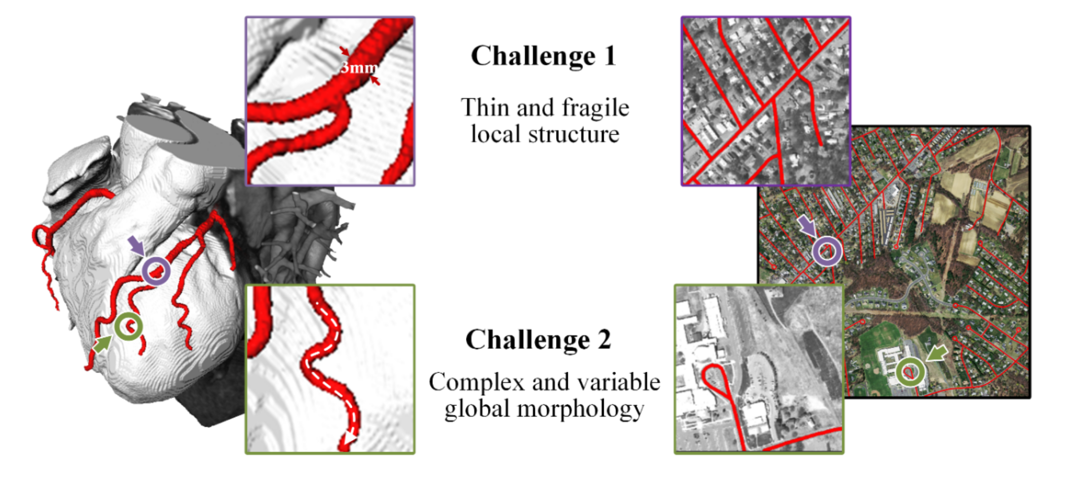
1. Thin and fragile local structure. As is illustrated above, such structures account for only a small proportion of the overall image, and are susceptible to interference from backgrounds.
2. Complex and variable global morphology. Morphological variations are observed in targets located in different regions, depending on the number of branches, the location of bifurcations, and the path length. The model is likely to overfit on these features, resulting in weak ability to generalize.

With the recent emergence and prevalence of large models for computer vision tasks (e.g., SAM), which have exhibited excellent performance in basic tasks like segmentation, it seems that there is gradually forming a paradigm: people tend to fine-tune such models to adapt to the specific downstream tasks. At this point, it is controversial whether specified models, in contrast to large, general ones, are still worthwhile to be designed.

From a personal perspective, I opine that models particularly designed and implemented for certain tasks are still worth much attention. Here are 2 reasons:

1. For complex tasks like tubular structure segmentation proposed in this paper, large models may have the potential to cover them, while it takes too much time and energy to be tuned for such tasks in most cases.
2. Most large models in NLP and CV currently lack convincing interpretability, which might be easier to endow in terms of small, specified models.

To sum, this work proposed a novel framework of knowledge fusion to address the difficulties of segmenting thin tubular structures. The specific contributions are three-fold:

1. A dynamic snake convolution was proposed to adaptively focus on the slender and tortuous local features and realize the accurate tubular structures segmentation on both 2D and 3D datasets.
2. A multi-perspective feature fusion strategy was proposed to supplement the attention to the vital features from multiple perspectives.
3. A topological continuity constraint loss function based on Persistent Homology was proposed, which better constrains the continuity of the segmentation.

Methodology

Though designed for both 2D and 3D feature maps for thin tubular structures, the methodology is described only in 2D situation for simplicity.

Dynamic Snake Convolution

Given the standard 2D convolution coordinates as $K$, with the central coordinate being $K_i=(x_i, y_i)$, a $3\times 3$ kernel $K$ with dilation rate 1 denotes as

Inspired by Deformable Convolutional Networks, deformation offsets $\Delta$ are introduced to make the kernel more flexible when focusing on complex geometric features of the target.

We may first start with the original deformable convolution.

Deformable Convolution

CNNs are inherently limited to model large, unknown transformations. The limitation originates from the fixed geometric structures of CNN modules:

• a convolution unit samples the input feature map at fixed locations
• a pooling layer reduces the spatial resolution at a fixed ratio
• a RoI (region-of-interest) pooling layer separates a RoI into fixed spatial bins
• …

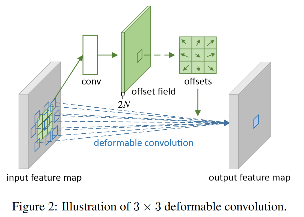
So in paper Deformable Convolutional Networks, the authors proposed integrating learnable 2D offsets with the regular grid sampling locations in the standard convolution, as depicted below.

Here this work mentioned:

However, if the model is left free to learn the deformation offsets, the perceptual field tends to stray outside the target, especially in the case of thin tubular structures.

Therefore, we use an iterative strategy, selecting the following position to be observed in turn for each target to be processed, thus ensuring continuity of the attention and not spreading the field of sensation too far due to the large deformation offsets.

In short, all offsets are learned at once, and the only constraint on the offsets is the size of receptive field. So this is a relatively “free” learning process. Such “freedom” may lead to loss on details, which could be especially horrible for our task of thin tubular structure segmentation.

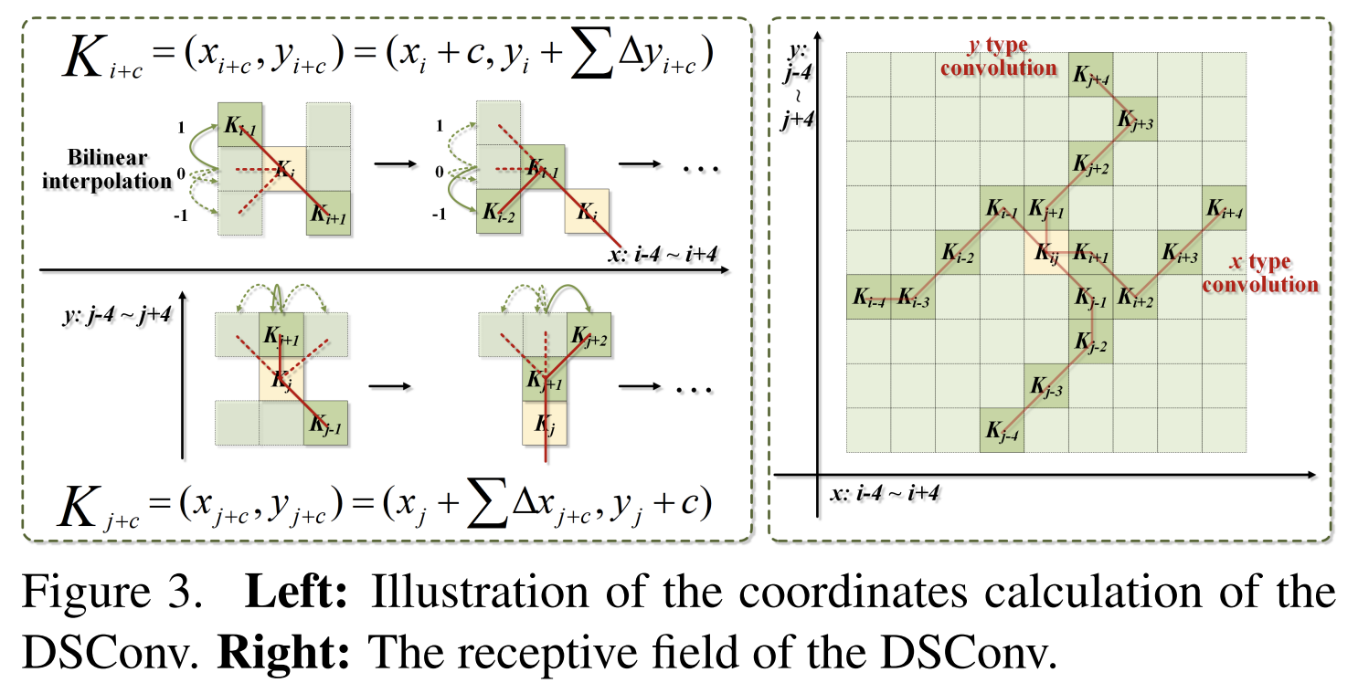
In DSConv, the standard convolution kernel is straighten both in the direction of x- and y-axis. The selection of each grid position $K_{i\pm c}$ in the kernel is a cumulative process: Starting from the center position $K_i$, the position away from the center grid depends on the position of the previous grid: $K_{i+1}$ is augmented with an offset $∆ = {δ|δ ∈ [−1, 1]}$ compared to $K_i$. Intuitively, this poses constraints on the cotinuity of the offsets; therefore, each grid chooses its direction based on its former grid.

Multi-view Feature Fusion Strategy

This part is relatively simple. It proposed random dropping to solve possible overfitting problems and reduce memory usage when intergating essential features from multiple perspectives.

I may replenish this part later, if anything important is missed.

Topological Continuity Constraint Loss

Compared to Wasserstein distance, which may have some problem with outlier points, here the authors adopted the more robust Hausdorff distance to measure the distance between to sets. This is simple, but the real question is:

Let’s first get down to a new concept: Persistent Homology, PH for short.

Persistent Homology: a Brief Introduction

PH is applied to compute the evolution of topological features, and the period between the appearance time $b$ and disappearance time $d$ of topological features is kept.

Such periods are summarized in a concise format called a persistence diagram (PD), which consists of a set of points $(b, d)$. Each point $(b, d)$ represents the $d$-th homology class ¹ that appears at $b$ and disappears at $d$.

Let $PD = dgm(·)$ denote the persistent homology obtained from the groundtruth $L$ and prediction $O$. We consider the topological information in complex tubular structures, which contains the key clues to determine the presence of fractures, to be evident in the homotopy features of 0-dimensional and 1-dimensional homological features.

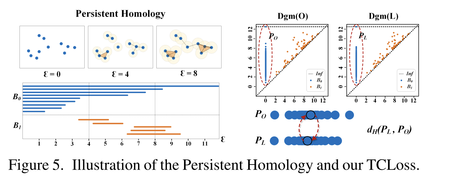
Now consider Hausdorff distance, and we have

where $P_O ∈ dgm(O)$ , $P_L ∈ dgm(L)$ and $d^*_H$ represents the bidirectional Hausdorff distance, which is computed in terms of n-dim points.