Origin Ensemble PET Reconstruction
Published:
The origin ensemble (OE) algorithm is a novel statistical method for MMSE reconstruction of emission tomography data. This method allows one to perform reconstruction entirely in the image domain, i.e. without the use of forward and backprojection operations.
Formulation
MMSE PET reconstruction
MMSE = Minimum-mean-square-error
PET imaging can be described as $I\times J$ Poisson variables $\mathbf{n}={n_{ij}}$ with expected value ${\lambda_{ij}}$
- $n_{ij}$ represents the number of annihilation events from voxel $i\in {1, \dots, I}$ detected by detector pair $j\in {1, \dots, J}$, which is unobservable
- The set composed of all the voxels is called image domain
- The set consisting all the detector pairs is called projection domain
The statistical relationship between the two domains is usually described by a system matrix ${\alpha_{ij}}$
- Element $\alpha_{ij}$ is the probability that event in voxel $i$ is detected by detector pair $j$
- Here the system matrix is supposed to be obtained from scanner geometry, and contains object-specific attenuation information already
In sum, the probability $\epsilon_i$ that the whole scanner detects an event from voxel $i$ can be denoted as
\[\epsilon_i=\sum\limits_{j}\alpha_{ij}, \tag{1}\]which is also called the sensitivity of voxel $i$
Let $\mathbf{\lambda}={\lambda_i}$ be the unknown, discrete emission density in image domain, where $\lambda_i$ is the emission counts in voxel $i$.
- Then the Poisson variable can be denoted as $\lambda_{ij}=\alpha_{ij}\lambda_{i}$
Considering the complete data $\mathbf{n}$, the likelihood for the estimation $\hat{\mathbf{\lambda}}={\hat{\lambda_i}}$ of emission density goes
\[\begin{aligned}\mathcal{L}(\hat{\lambda}|\mathbf{n})&=\mathcal{P}_{\hat{\lambda}}(\mathbf{n})=\prod\limits_{i, j}\frac{\hat{\lambda_{ij}}^{n_{ij}}}{n_{ij}!}e^{-\hat{\lambda_{ij}}}\\ \hat{\lambda_{ij}}&=\alpha_{ij}\hat{\lambda_i}\end{aligned}. \tag{2}\]However, data acquired in real-world are usually incomplete, say $\mathbf{n}^{\ast}={n^{\ast}_j}$. We need to estimate emission density $\lambda$ from the incomplete data.
\[n^{\ast}_j=\sum\limits_in_{ij}. \tag{3}\]Eventually, our estimation is as follows
\[\mathbf{\hat{\lambda}}^{(\text{ML})}={\arg\max}_{\mathbf{\hat{\lambda}}}\mathcal{L}(\mathbf{\hat{\lambda}}|\mathbf{n}^{\ast}), \tag{4}\]wherein $\mathbf{\hat{\lambda}}^{(\text{ML})}$ is usually calculated iteratively, e.g., EM-type algorithms like MLEM and OSEM
A particular characteristic of such techniques is their use of FP of the image estimate to the projection domain, which allows to compare the estimated projection data with the acquired projection data. In turn, BP of adequate correction terms is used to amend the image estimate accordingly. Successive FP and BP are repeated a certain number of times, or until a predefined convergence criterion is met.
Different from FP/BP-driven methods above, origin ensemble algorithm directly estimates the emission counts in each voxel $i$.
\[n_i=\sum\limits_jn_{ij}. \tag{5}\]The MMSE estimation about the emission counts in each voxel $i$ can be denoted as
\[E[n_i|\mathbf{n^{\ast}}]=\sum\limits_{\mathbf{\hat{n}}\in \Theta}n_i(\mathbf{\hat{n}})\mathcal{P}(\mathbf{\hat{n}}|\mathbf{n^{\ast}}), \tag{6}\]Finally, emission counts in voxel $i$ can be derived by dividing sensitivity $\epsilon_i$
\[\hat{\lambda}_i^{(MMSE)}=\begin{cases}E[n_i|\mathbf{n^{\ast}}]/\epsilon_i, \text{for} \thinspace \epsilon_i>0\\0, \text{for}\thinspace \epsilon_i=0\end{cases}. \tag{7}\]Origin Ensemble
By allocating each detected event $k$ to voxel $i_k$ with probability $\alpha_{i_kj_k}>0$, we can obtain complete data set $\mathbf{\hat{n}}\in \Theta$ from acquired data $\mathbf{n^{\ast}}$
We define origin ensembles as configurations of the events detected in image domain, denoted as
\[\mathbf{\omega}=\left\{(i_1, j_1), \dots, (i_k, j_k), \dots\right\}\in \Omega, \tag{8}\]where $\Omega$ represents all possible OEs, called OE domain.
Given an OE $\mathbf{\omega}\in \Omega$, let $n_i(\mathbf{\omega})$ be the emission counts allocated to voxel $i$. Then its MMSE estimation writes as
\[\begin{aligned}E[n_i|\mathbf{n^{\ast}}]&=\sum\limits_{\mathbf{\hat{n}}\in\Theta}n_i(\mathbf{\hat{n}})\mathcal{P}(\mathbf{\hat{n}}|\mathbf{n^{\ast}})\\&=\sum\limits_{\mathbf{\hat{n}}\in\Theta}\left\{\sum\limits_{\omega\in\Omega}\mathcal{P}(\mathbf{\hat{n}}|\omega, \mathbf{n^{\ast}})\mathcal{P}(\omega|\mathbf{n^{\ast}})\right\}\\&=\sum\limits_{\omega\in\Omega}\left\{\sum\limits_{\mathbf{\hat{n}}\in\Theta}n_i(\mathbf{\hat{n}})\mathcal{P}(\mathbf{\hat{n}}|\omega)\right\}\mathcal{P}(\omega|\mathbf{n^{\ast}})\\&=\sum\limits_{\omega\in\Omega}n_i(\omega)\mathcal{P}(w|\mathbf{n^{\ast}})\end{aligned}. \tag{9}\]Above all, we have the following conclusions:
- the MMSE estimation for emission counts can be obtained by averaging over the OE domain with weights, rather than complete data domain $\Theta$
- what remains unknown:
- expression for the posterior in Eq. (9)
- effective algorithmic methods to compute MMSE estimation
OE posterior
Exploring the statistical relationship between OE $\omega\in \Omega$ and its corresponding complete data set $\mathbf{\hat{n}}(\omega)\in \Theta$
By applying Bayes’ theorem and marginalizing $\lambda$ out, the posterior probability of OE complete data $n$ transforms to
\[\begin{aligned} \mathcal{P}\left(\boldsymbol{n} \mid \boldsymbol{n}^*\right)&=\frac{\mathcal{P}\left(\boldsymbol{n}^* \mid \boldsymbol{n}\right) \mathcal{P}(\boldsymbol{n})}{\mathcal{P}\left(\boldsymbol{n}^*\right)}\\ &=\frac{\mathcal{P}\left(\boldsymbol{n}^* \mid \boldsymbol{n}\right)}{\mathcal{P}\left(\boldsymbol{n}^*\right)} \int_{\boldsymbol{\lambda}} \mathcal{P}_{ \boldsymbol{\lambda}}(\boldsymbol{n}) \mathrm{d} \mathcal{P}(\boldsymbol{\lambda}) \end{aligned} , \tag{10}\]Based on Eq. (2), the posterior can de separated into 2 parts. The former part is only related to $\mathbf{n}$, while the latter is conditioned on both $\mathbf{n}$ and $\mathbf{\lambda}$, denoted as $\mathcal{P}_{ \boldsymbol{\lambda}}(\boldsymbol{n})=\varphi(\boldsymbol{n})\psi(\boldsymbol{\lambda}, \boldsymbol{n})$, wherein
\[\begin{aligned}\varphi(\boldsymbol{n})&=\prod_{i, j}\frac{\alpha_{ij}^{n_{ij}}}{n_{ij}!}\\\psi(\boldsymbol{\lambda}, \boldsymbol{n})&=\prod_i\lambda_i^{n_i}e^{-\epsilon_i\lambda_i}\end{aligned}. \tag{11}\]By inserting $\varphi$ and $\psi$ into Eq. (10), we arrive at
\[\mathcal{P}\left(\boldsymbol{n} \mid \boldsymbol{n}^*\right) \propto \varphi(\boldsymbol{n}) \int_{\boldsymbol{\lambda}} \psi(\boldsymbol{\lambda}, \boldsymbol{n}) \mathrm{d} \mathcal{P}(\boldsymbol{\lambda}). \tag{12}\]For simplification, a flat prior is used for $\mathcal{P}(\boldsymbol{\lambda})$; considering Gamma distribution, here we have
\[\mathcal{P}_{\mathrm{f}}\left(\boldsymbol{n} \mid \boldsymbol{n}^*\right) \propto \varphi(\boldsymbol{n}) \prod_i \frac{n_{i} !}{\varepsilon_i^{n_i}}. \tag{13}\]So far, it can be ensured that all the parameters are known. But there are two problems unsolved yet:
- too much cost on computation
- Eq. (9) needs the posterior of an OE $\omega$, rather than that of complete data $\mathbf{n}$. And for a complete data set $\mathbf{n}$, there are often multuple OEs $w_1, \dots, w_D$ that corresponds to it.
Q1 is left in Algorithmic methods part. Here we first consider Q2.
An Example
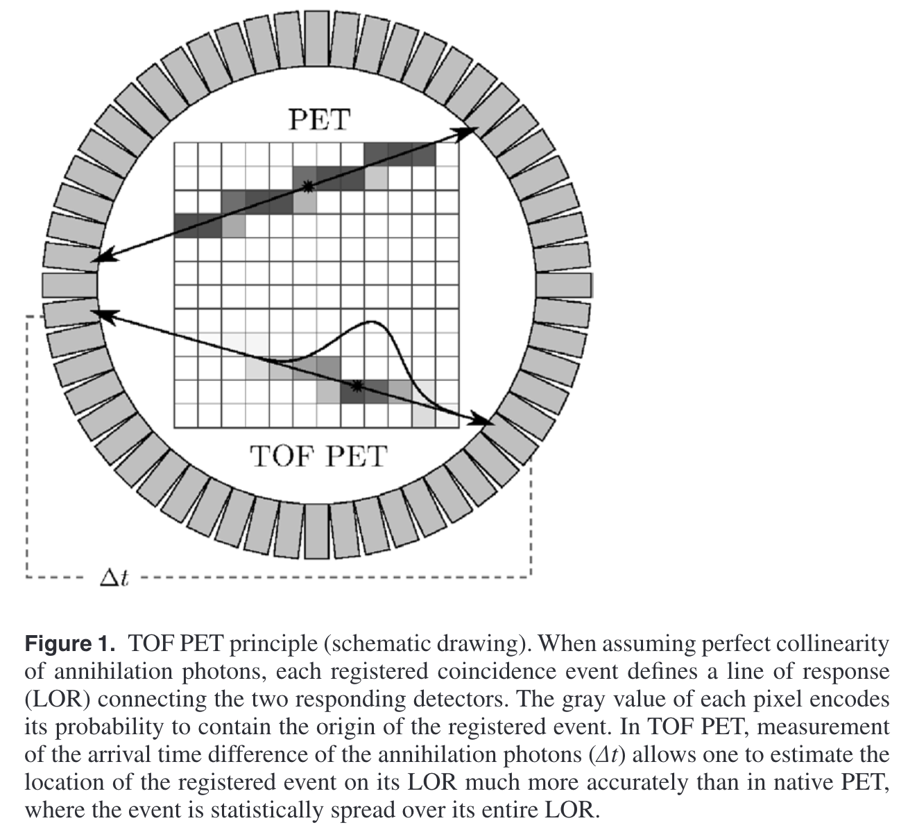
Take the example of PET imaging system with 4 detectors and 4 voxels, as illustrated in the figure below.
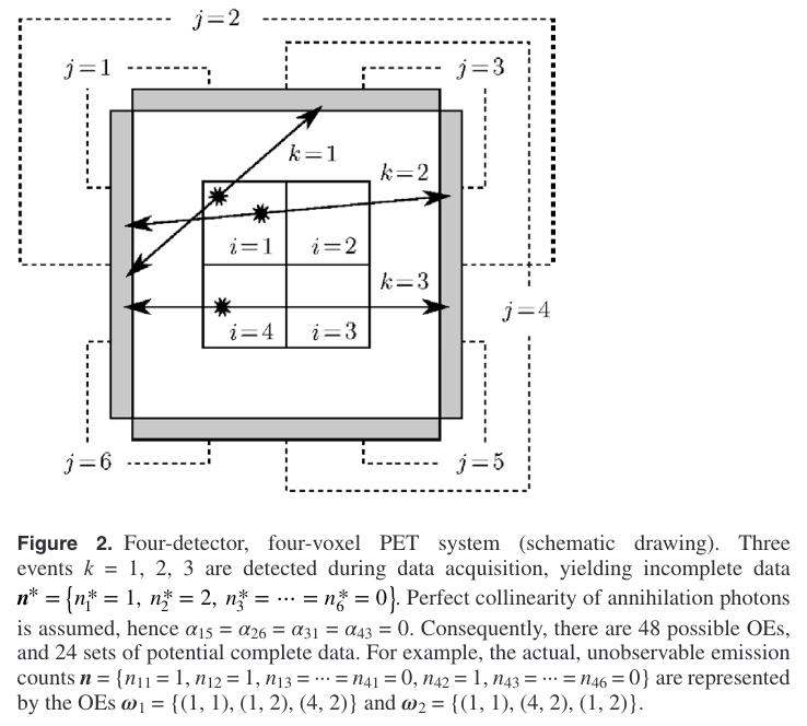
There are 3 registered events $k=1, 2, 3$, wherein event $k=1$ is detected by pair $j=1$, while events $k=2, 3$ are detected by $j=2$. Then the incomplete data acquired is
\[\boldsymbol{n}^*=\left\{n_1^*=1, n_2^*=2, \cdots, n_6^*=0\right\}. \nonumber\]To simplify, perfect collinearity is assumed, i.e., $\alpha_{15}=\alpha_{26}=\alpha_{31}=\alpha_{43}=0$.
Therefore, event $k=1$ can occur in voxel $i=1, 2, 4$, whereas events $k=2, 3$ can occur in voxel $i=1, 2, 3, 4$. There are $3\times4\times4=48$ possible OEs $\omega={(i_1, j_1), (i_2, j_2), (i_3, j_3)}$ altogether, where $i_1, i_2, i_3$ denotes positions of voxels, and $j_1, j_2, j_3$ are corresponding detector pairs.
Note that we can swap voxel positions of events $k=2, 3$ to obtain 2 different OEs, i.e.,
$\omega_1={(1, 1), (1, 2), (4, 2)}$
$\omega_2={(1, 1), (4, 2), (1, 2)}$
and they are equiprobable.
Generally, for each potential complete data $\boldsymbol{n} \in \Theta$, there are in total
\[D=\prod_j \frac{n_j^{*} !}{\prod\limits_i n_{i j} !}\tag{14}\]equiprobable OEs $\omega_1, \dots, \omega_D$. So we can arrive at the following statistical relationship
\[\mathcal{P}(w_1|\boldsymbol{n}^*)=\cdots=\mathcal{P}(w_D|\boldsymbol{n}^*)=D^{-1}\mathcal{P}(\boldsymbol{n}|\boldsymbol{n}^*). \tag{15}\]Combining with Eq. (11), (13), (14), (15), the computation-demanding term $n_{ij}!$ can be reduced. Thus there is
\(\mathcal{P}_{\mathrm{f}}\left(\boldsymbol{\omega} \mid \boldsymbol{n}^*\right) \propto \prod_i \frac{n_{i} !}{\varepsilon_i^{n_i}} \prod_j \alpha_{i j}^{n_{i j}}. \tag{16}\) Now we have the expression Eq. (16) that calculates the posterior of OE not relying on any prior.
Algorithmic methods
OE reconstruction with Metropolis-Hastings sampling
In reality, there are often $10^6\sim 10^7$ registered events, and the number of voxels is on the order of $10^5\sim 10^6$. Naïvely veraging over the whole OE domain $\Omega$ is not possible. MCMC methods can overcome this obstacle; specifically, we can neglect OEs that have a low posterior in Eq. (9), thus using a manageable number of OEs to perform reconstruction.
Consider a sequence of OEs
\[\omega_0, \omega_1, \omega_2,\cdots. \tag{17}\]Let the equilibrium distribution be $\mathcal{P}(\cdot\mid\boldsymbol{n}^*)$ , i.e., the OE posterior.
Metropolis-Hastings sampling method is suitable for this problem, since it only requires a multiplicative constant for the target distribution. Specifically, based on the current state $\omega$, a random new state $\omega^{\prime}\in \Omega$ is picked from proposal distribution
\[Q(\cdot \mid \boldsymbol{\omega}): \Omega \rightarrow[0,1], \quad \boldsymbol{\omega}^{\prime} \mapsto Q\left(\boldsymbol{\omega}^{\prime} \mid \boldsymbol{\omega}\right). \tag{19}\]Proposed new state is accepted with an acceptance probability
\[A(\omega^{\prime}\mid\omega)\in [0, 1]. \tag{20}\]If the proposed new state is rejected, it stays at the current state. Here we use the standarad Metropolis acceptance probability
\[A\left(\boldsymbol{\omega}^{\prime} \mid \boldsymbol{\omega}\right)=\min \left\{1, \frac{\mathcal{P}\left(\boldsymbol{\omega}^{\prime} \mid \boldsymbol{n}^*\right)}{\mathcal{P}\left(\boldsymbol{\omega} \mid \boldsymbol{n}^*\right)} \cdot \frac{Q\left(\boldsymbol{\omega} \mid \boldsymbol{\omega}^{\prime}\right)}{Q\left(\boldsymbol{\omega}^{\prime} \mid \boldsymbol{\omega}\right)}\right\}, \tag{21}\]wherein $Q\left(\boldsymbol{\omega} \mid \boldsymbol{\omega}^{\prime}\right)$ is the probability to propose a transition to state $\omega$ when the Markov chain is in state $\omega^{\prime}$, vice versa for $Q\left(\boldsymbol{\omega}^{\prime} \mid \boldsymbol{\omega}\right)$.
Usually, state proposal and stochastic acceptance would be repeated many times to ensure that the chain is aperiodic; so is the proposal distribution $Q$, to ensure that the chain is irreducible on $\Omega$. Therefore, uniqueness of and convergence to the equilibrium distribution are guaranteed.
For a single event $k$, $\mathcal{P}$ in Eq. (21) can be simplified as
\[\frac{\mathcal{P}_{\mathrm{f}}\left(\boldsymbol{\omega}^{\prime} \mid \boldsymbol{n}^*\right)}{\mathcal{P}_{\mathrm{f}}\left(\boldsymbol{\omega} \mid \boldsymbol{n}^*\right)}=\frac{\alpha_{i^{\prime} j_k}}{\alpha_{i j_k}} \cdot \frac{\varepsilon_i}{\varepsilon_{i^{\prime}}} \cdot \frac{n_{i^{\prime}}(\boldsymbol{\omega})+1}{n_i(\boldsymbol{\omega})}. \tag{22}\]In addition, it’s obvious that any state $\hat{\omega}\in \Omega$ can be reached by moving each event $k=1, \dots, K$ to the given positions in $\hat{\omega}$ from other states $\omega\in \Omega$. Hence, we repeat state proposal and stochastic acceptance $K$ times (i.e., as many as the number of events), to ensure the aperiodicity and irreducibility of the chain.
Integrating TOF information
Take 2-dimensional pixelized plane as an example, so that each detector pair $j$ can be described as an LOR (Line of Response).
Each LOR $j$ is determined by its two endpoints $\boldsymbol{x}_j^{(1)}, \boldsymbol{x}_j^{(2)}\in\mathbb{R}^2$. So here comes its parametrized definition
\[\boldsymbol{\gamma}_j:[0,1] \rightarrow \mathbb{R}^2, \quad t \mapsto \boldsymbol{x}_j^{(1)}+t \cdot\left\{\boldsymbol{x}_j^{(2)}-\boldsymbol{x}_j^{(1)}\right\}. \tag{23}\]Next, we focus on element $\alpha_{ij}$ in system matrix, which integrates the TOF information in reconstruction.
- in reality, due to the fact that system matrix is large and sparse, not easy to store, its elements are calculated real-time
- the calculation of an element $\alpha_{ij}$ is based on the length of the segment of LOR $j$ that locates in pixel $i$, denoted as $l_{ij}$. So we have
\(\alpha_{ij}\propto l_{ij}=\int_{\boldsymbol{\gamma}_j}1_i\mathrm{d} s, \tag{24}\) where $1_i$ is the indicator function for pixel $i\in \mathbb{R}^2$.
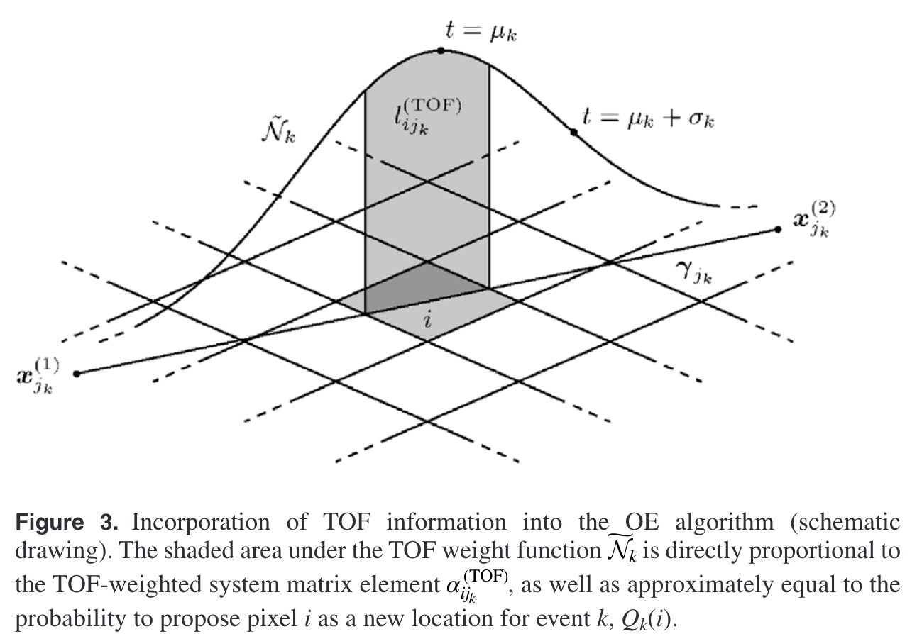
Integration of TOF information can be achieved via adding a TOF-weighted function $\widetilde{\mathcal{N}}_k$ to the LOR of each event $k$. $\widetilde{\mathcal{N}}_k$ can be approximated via Gaussian
\[\widetilde{\mathcal{N}}_k\left(\boldsymbol{\gamma}_{j_k}(t)\right) \approx \frac{1}{\sqrt{2 \pi \sigma_k^2}} \mathrm{e}^{-\frac{1}{2}\left[\frac{t-\mu_k}{\sigma_k}\right]^2}, \tag{25}\]wherein mean $\mu_k\in [0, 1]$ determines the most possible position of event $k$ on its LOR $j_k$, and standard deviation $\sigma_k$ is decided by both the length of LOR $j_k$ and TOF estimation accuracy of the scanner.
Eq. (24) then can be transformed to
\[\alpha_{i j_k}^{(\mathrm{TOF})} \propto l_{i j_k}^{(\mathrm{TOF})}=\int_{\gamma_{j_k}}\left(1_i \cdot \widetilde{\mathcal{N}}_k\right) \mathrm{d} s. \tag{26}\]By inserting the OE posterior in Eq. (22) into the acceptance probability $A$, a restraint on proposal distribution $Q_k$ can be derived as
\[Q_k(i)\propto l_{ij_{k}}^{(TOF)}\propto \alpha_{ij_k}^{TOF}\tag{27}\]Since Eq. (26) describes the dependence of $\alpha_{i j_k}^{(\mathrm{TOF})}$ upon volume element $i$ exclusively, Eq. (27) yields the cancellation of the proposal probabilities $Q_k(i)$ and $Q_k(i^{\prime})$ with the system matrix elements in the acceptance probability $A$, i.e.,
\[\frac{\alpha_{i^{\prime} j_k}^{(\mathrm{TOF})}}{\alpha_{i j_k}^{(\mathrm{TOF})}} \cdot \frac{Q_k(i)}{Q_k\left(i^{\prime}\right)}=1\tag{28}\]This can reduce the computational expense of the OE algorithm significantly.
For the Chinese version of this blog, please redirect to Origin Ensemble (Chinese ver.)